Introduction
In this multi-part series, we look inside LSTM forward pass. If you haven’t already read it I suggest run through the previous parts (part-1,part-2) before you come back here. Once you are back, in this article, we explore LSTM’s Backward Propagation. This would usually involve lots of math. I am not a trained mathematician, however, I have decent intuition. But just intuition can only get you so far. So I used my programming skills to validate pure theoretical results often cited by a pure mathematician. I do this using the first principles approach for which I have pure python implementation Deep-Breathe of most complex Deep Learning models.”
What this article is not about?
- This article will not talk about the conceptual model of LSTM, on which there is some great existing material here and here in the order of difficulty.
- This is not about the differences between vanilla RNN and LSTMs, on which there is an awesome post by Andrej if a somewhat difficult post.
- This is not about how LSTMs mitigate the vanishing gradient problem, on which there is a little mathy but awesome posts here and here in the order of difficulty.
What this article is about?
- Using the first principles we picturize/visualize the Backward Propagation.
- Then we use a heady mixture of intuition, Logic, and programming to prove mathematical results.
Context
This is the same example and the context is the same as described in part-1. The focus, however, this time is on LSTMCell.
LSTM Cell Backward Propagation
While there are many variations to the LSTM cell. In the current article, we are looking at LayerNormBasicLSTMCell. The next section is divided into 3 parts.
- LSTM Cell Forward Propagation(Summary)
- LSTM Cell Backward Propagation(Summary)
- LSTM Cell Backward Propagation(Detailed)
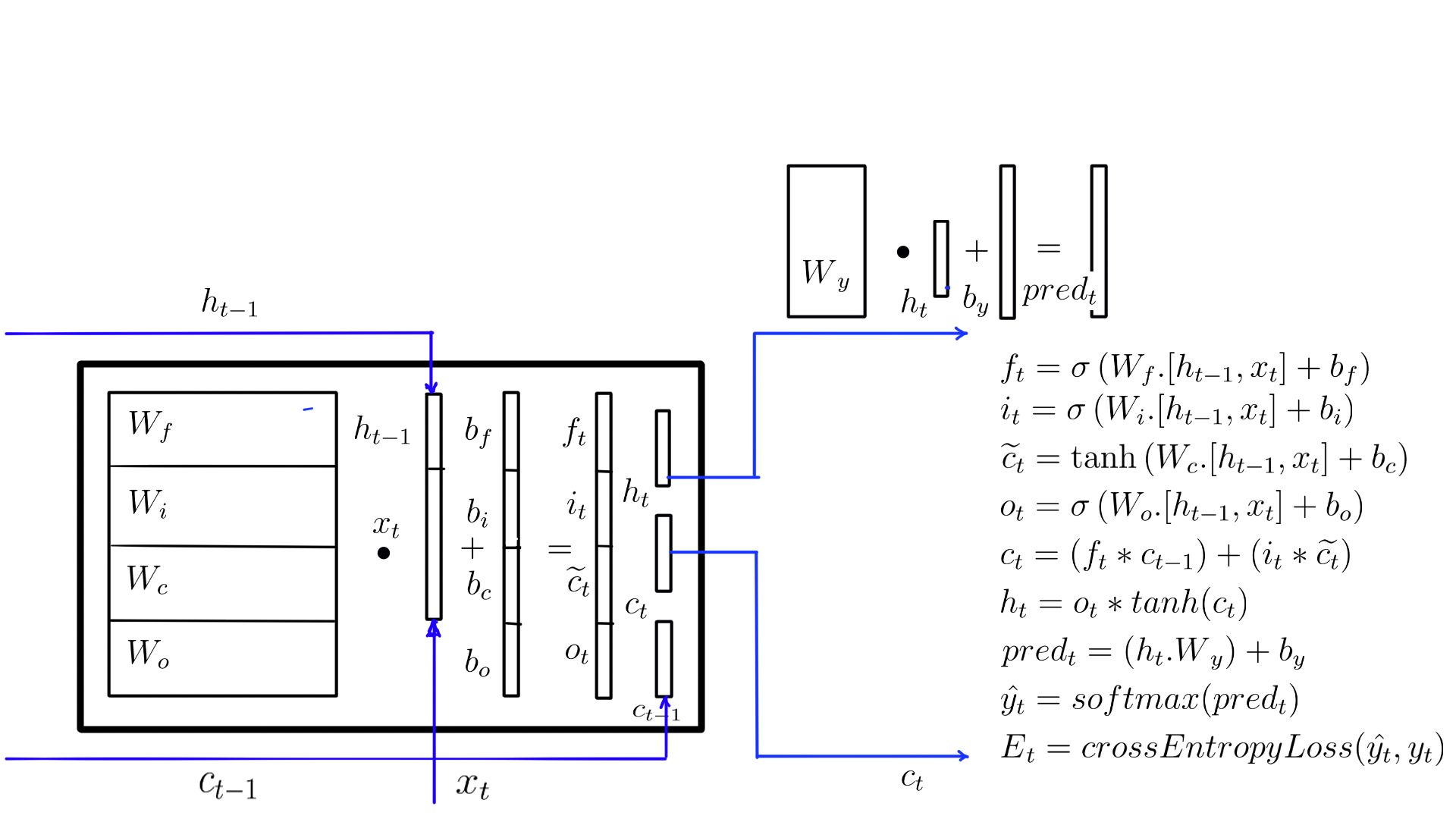
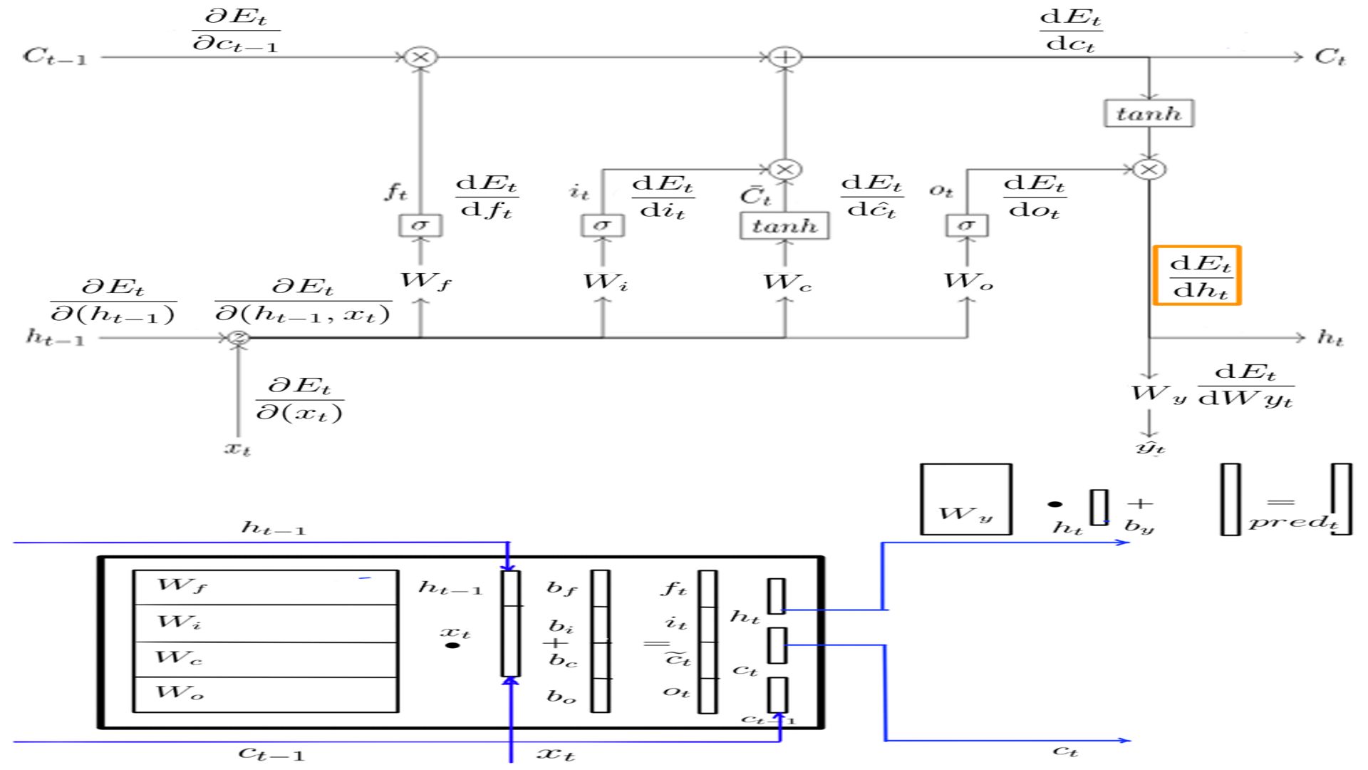
1. LSTM Cell Forward Propagation(Summary)
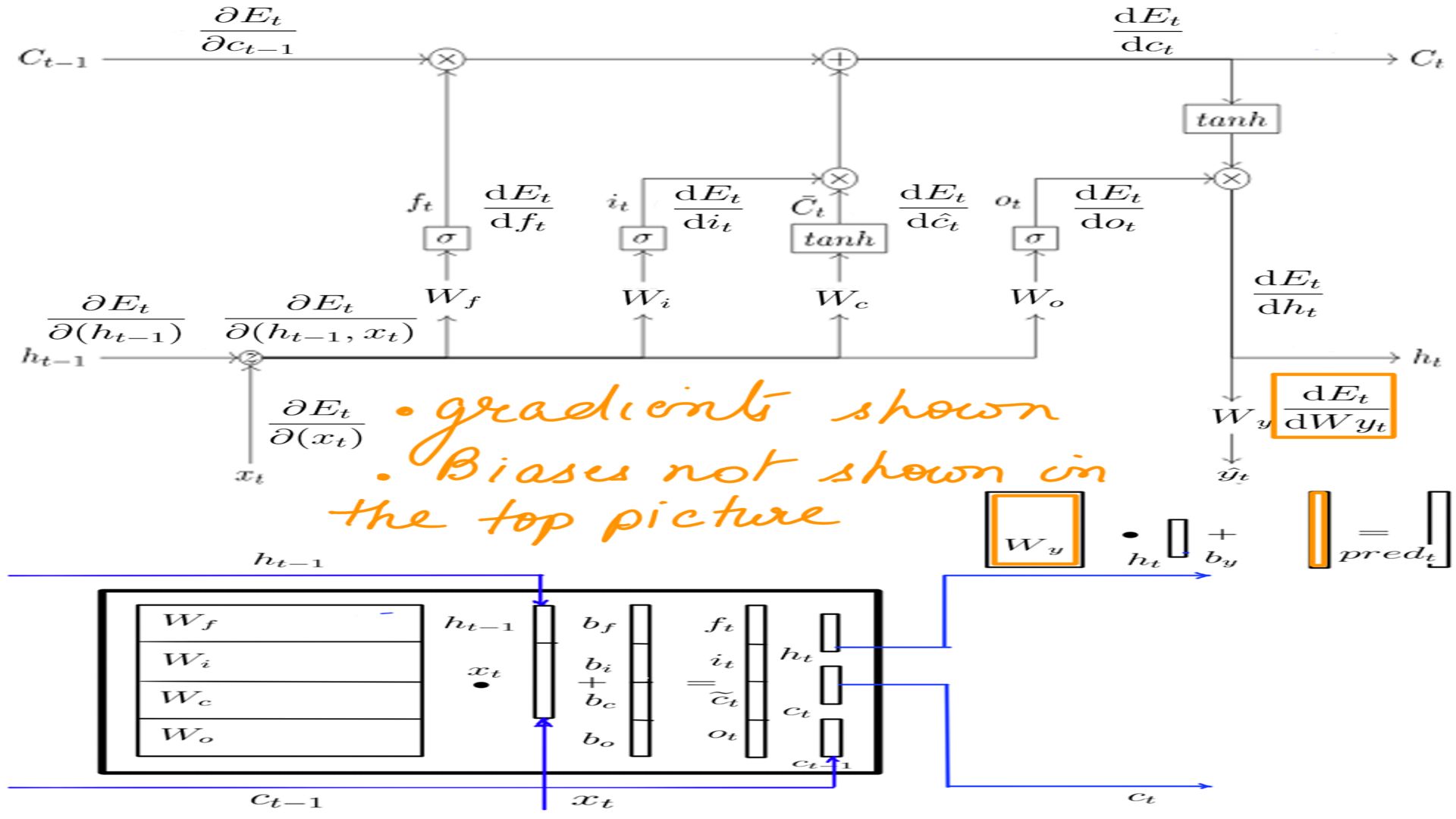
- Forward propagation:Summary with weights.
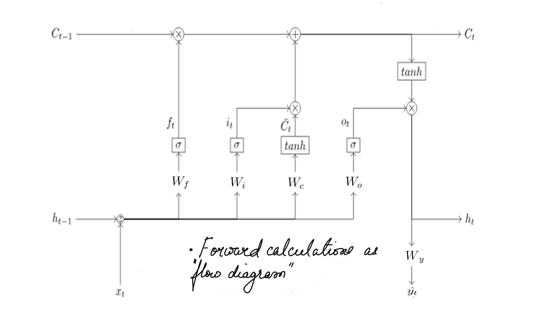
- Forward propagation:Summary as flow diagram.
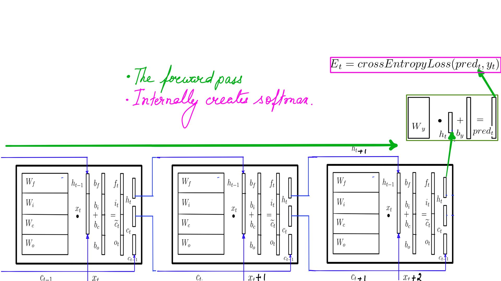
- Forward propagation: The complete picture.
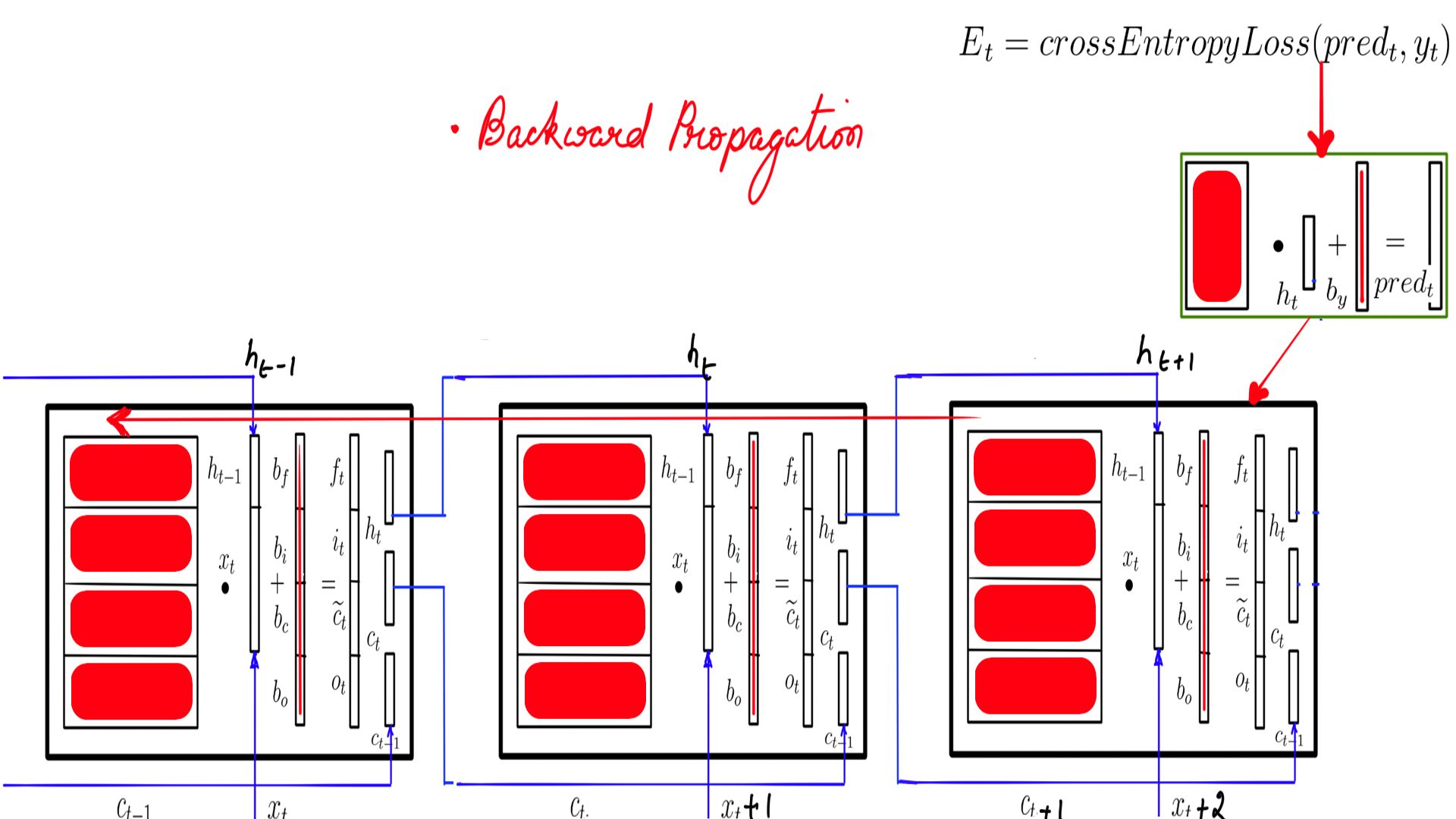
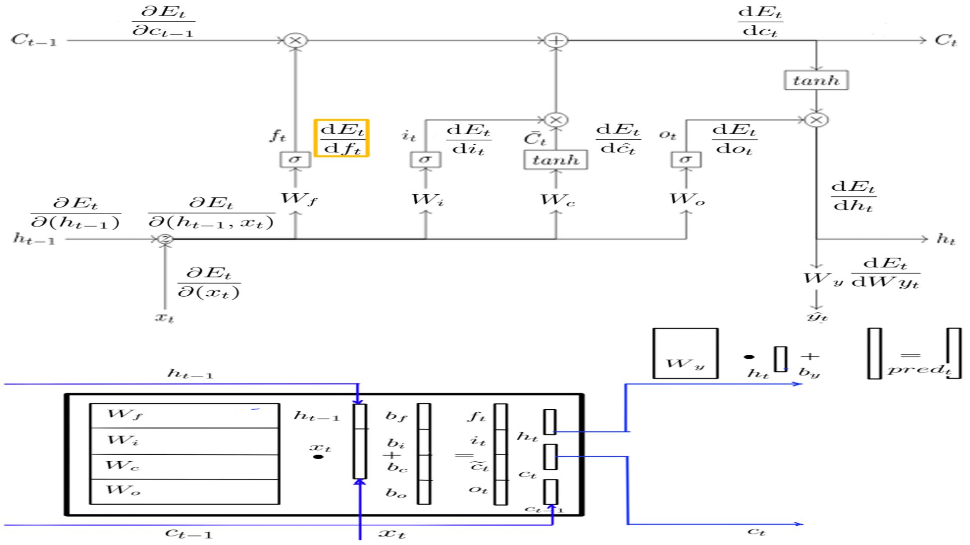
2. LSTM Cell Backward Propagation(Summary)
- Backward Propagation through time or BPTT is shown here in 2 steps.
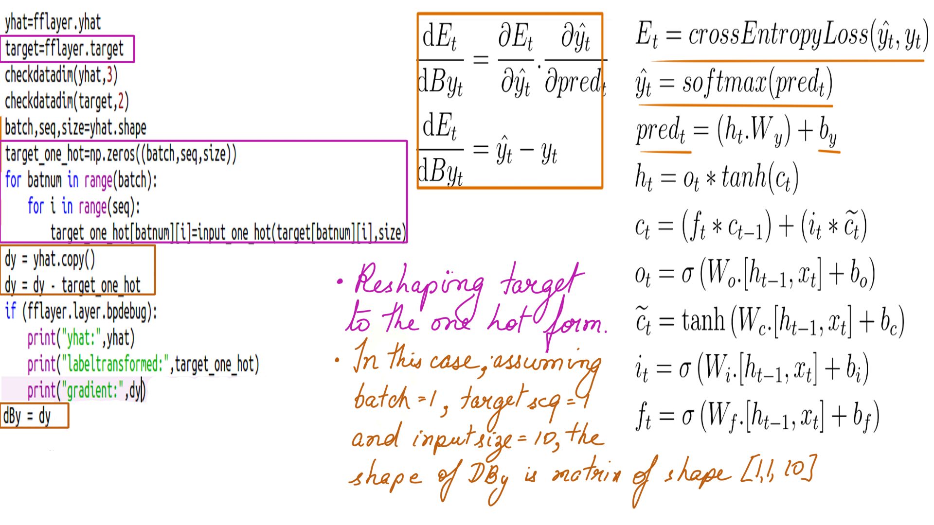
- Step-1 is depicted in Figure-4 where it backward propagates through the FeedForward network calculating Wy and By
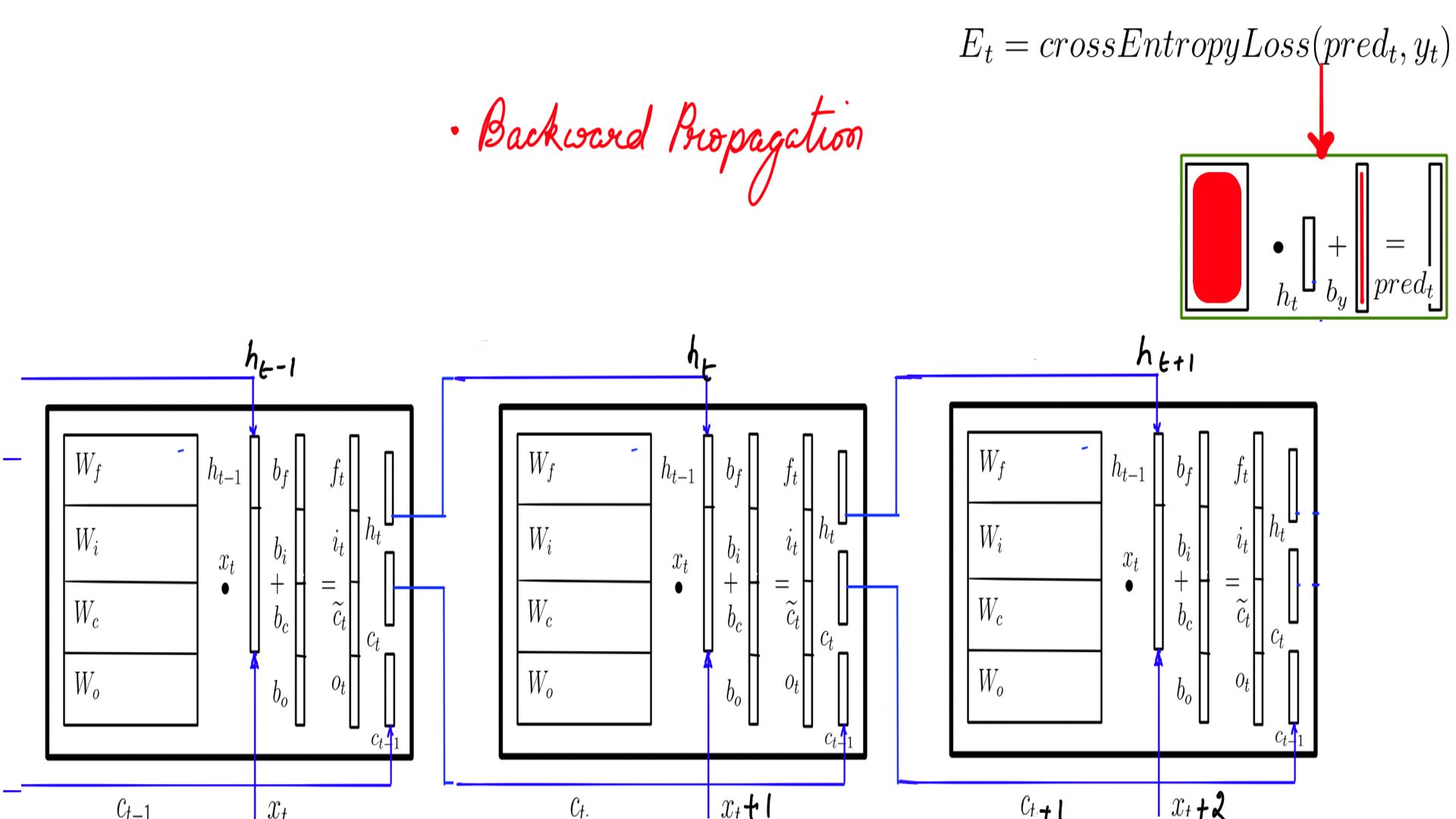
- Step-2 is depicted in Figure-5, Figure-6 and Figure-7 where it backward propagates through the LSTMCell. This is time step-3 or the last one. BPTT is carried out in reverse order.
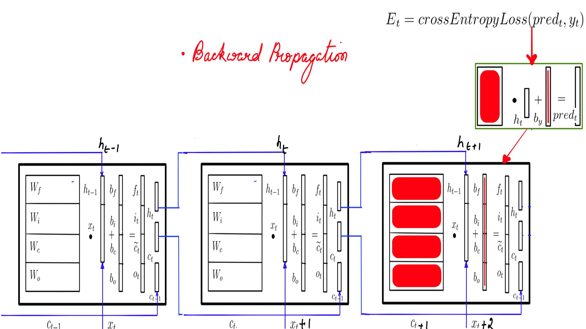
- Step-2 Repeat for remaining time steps in the sequence.
3. LSTM Cell Backward Propagation(Detailed)
The gradient calculation through the complete network is divided into 2 parts
Feed-Forward Network layer(Step-1)
- We have already done this derivation for “softmax” and “cross_entropy_loss”.
- The final derived form in eq-3. Which in turn depends on eq-1 and eq-2. We are calling it “pred” instead of “logits” in figure-5.
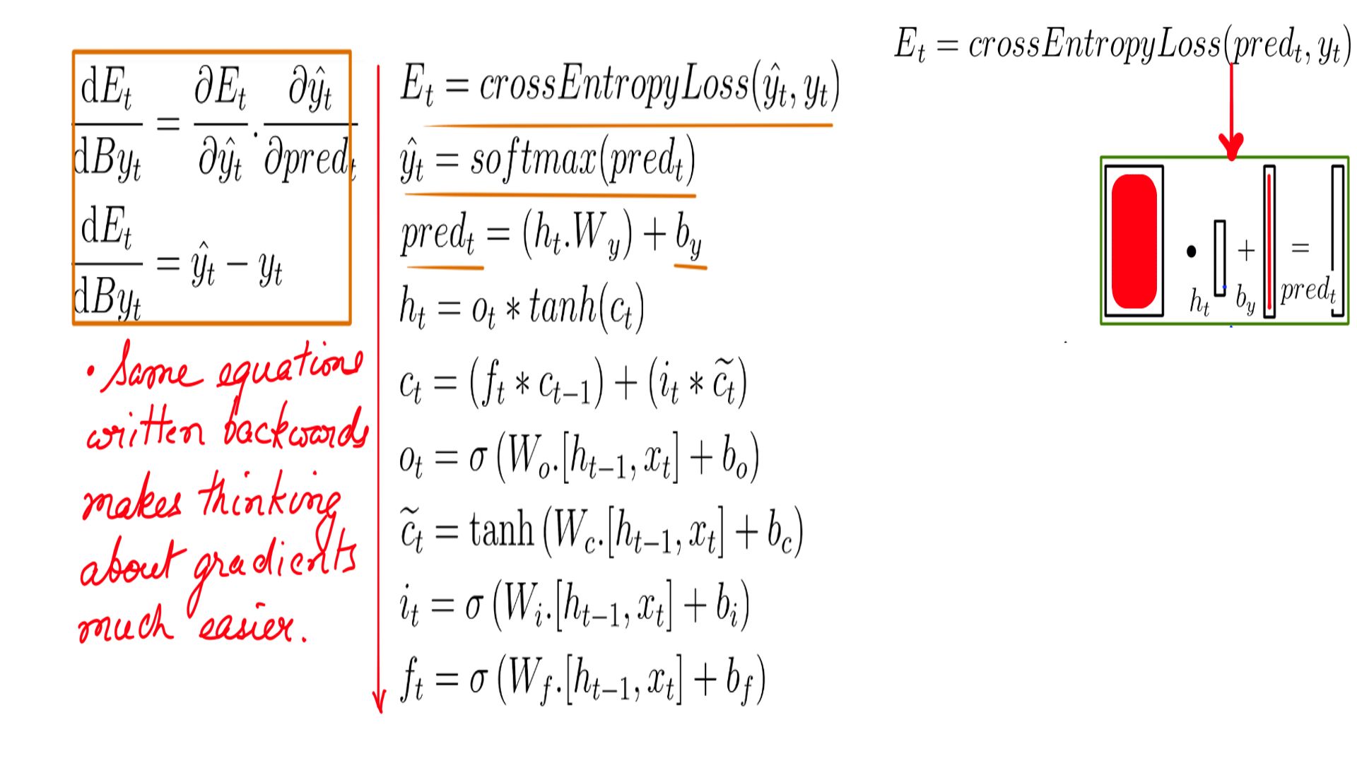
- “DBy” is straight forward, once the gradients for pred is clear in the previous step.
- This is just gradient calculation, the weights aren’t adjusted just yet. They will be adjusted together in the end as a matter of convenience by an optimizer such as GradientDescentOptimizer.
- The Complete code of listing can be found at code-1.
- “DWy” is straight forward too, once the gradients for pred is clear in the previous step(figure-5).
- The Complete code of listing can be found at code-2.
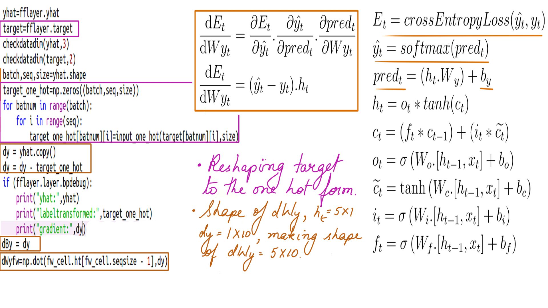
- “DWy” and “Dby”
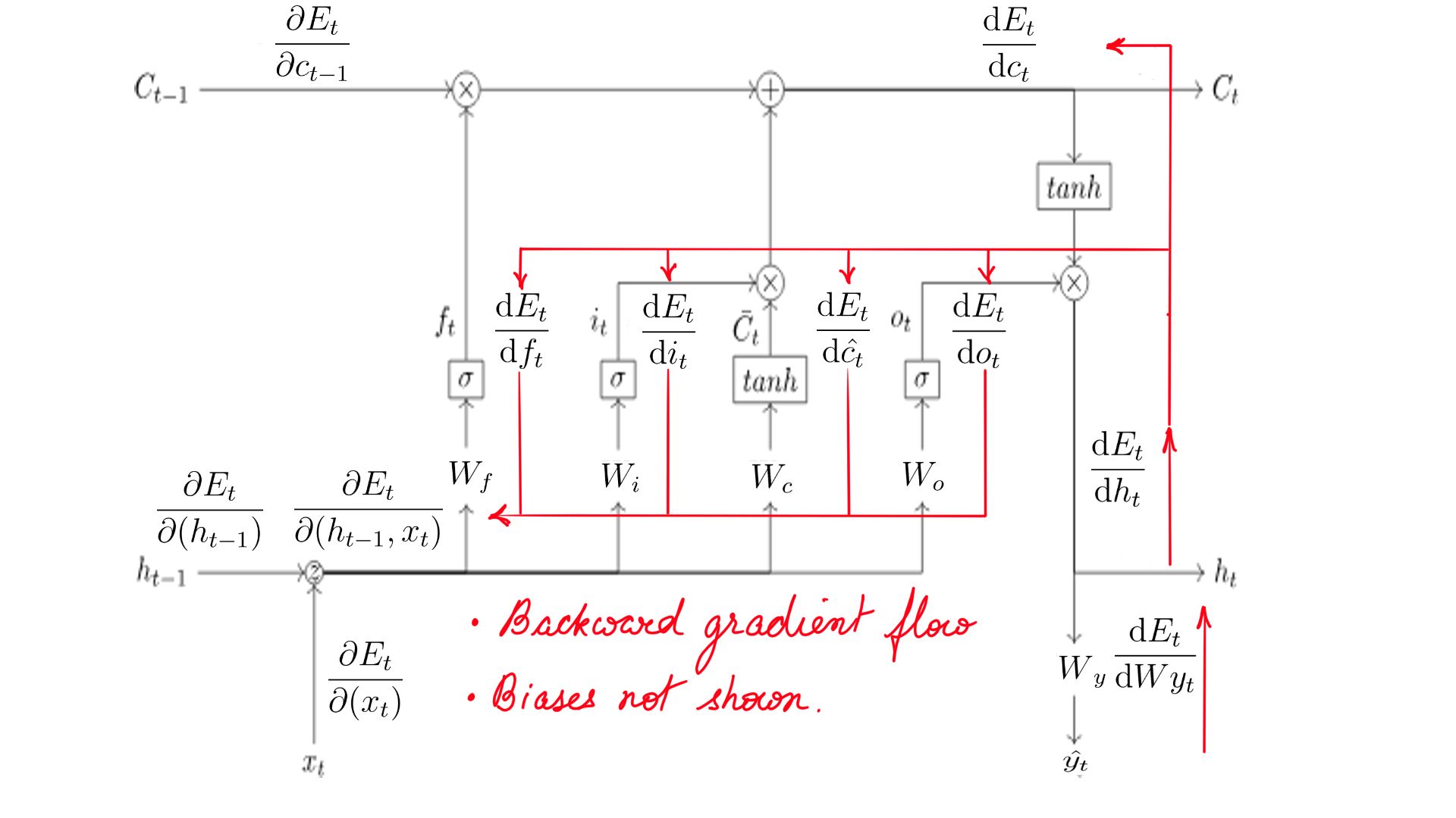
Backward propagation through LSTMCell(Step-2)
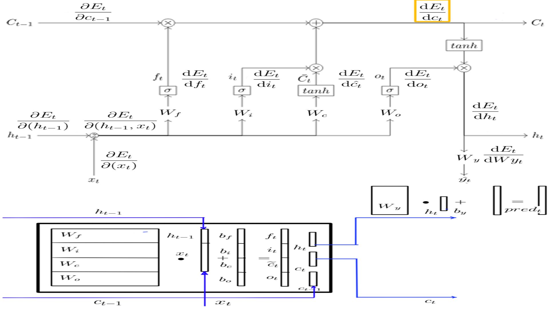
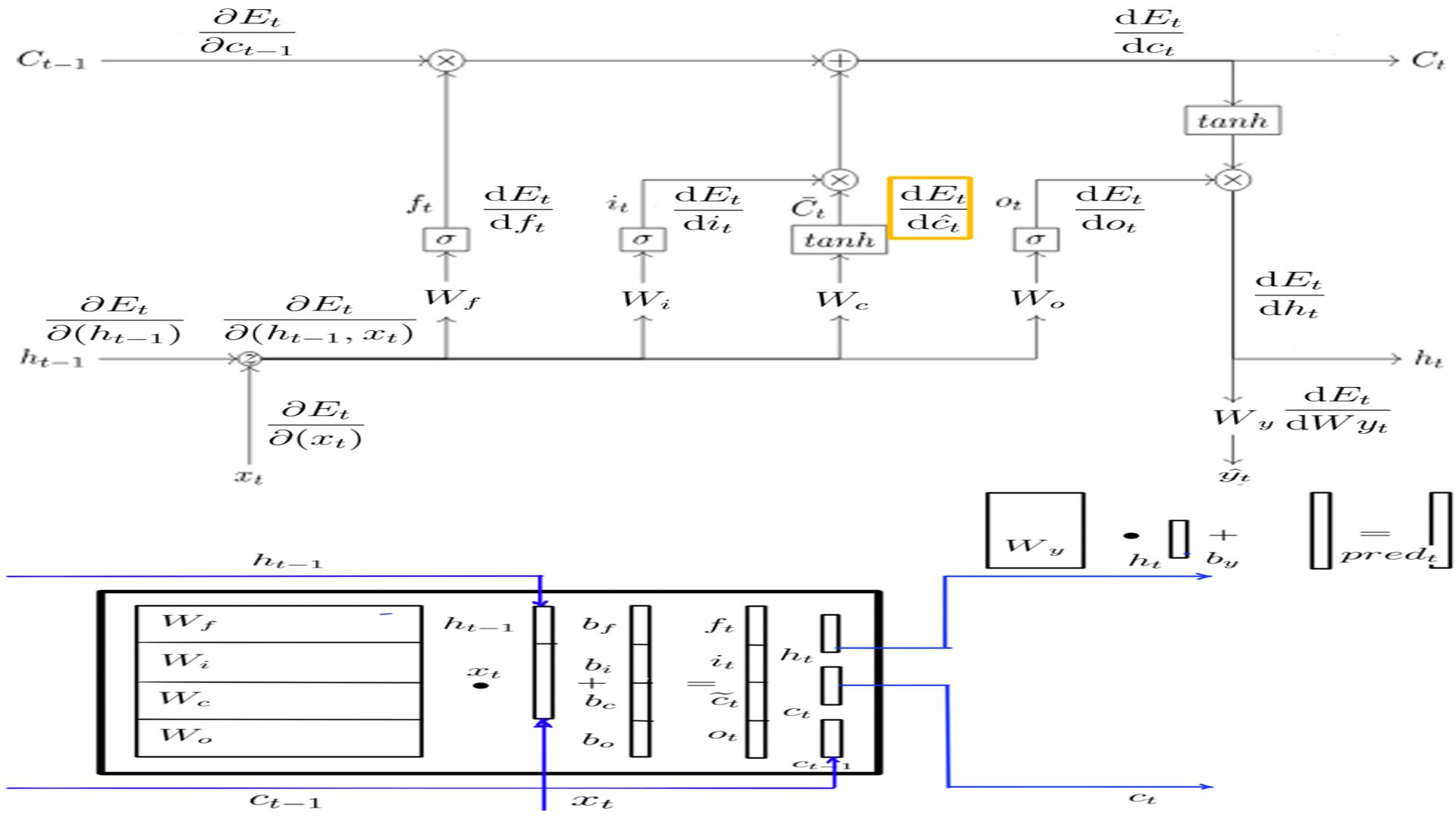
There are several gradients we are calculating, figure-6 has a complete list.
DHt
- Probably the most confusing step backward propagation because there is an element of time.
- There were 2 recursive elements h-state, c-state, similarly there 2 recursive elements while deriving the gradient backwards. We call it dh_next and dc_next, as you will see later both and many other gradients are derived from dHt.
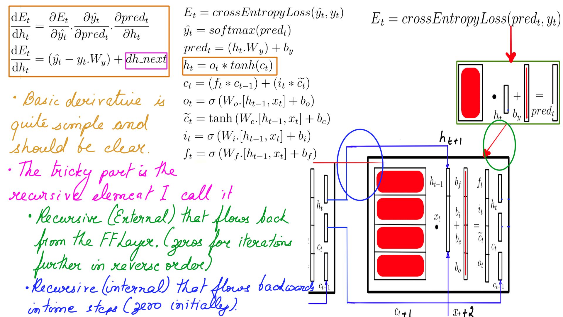
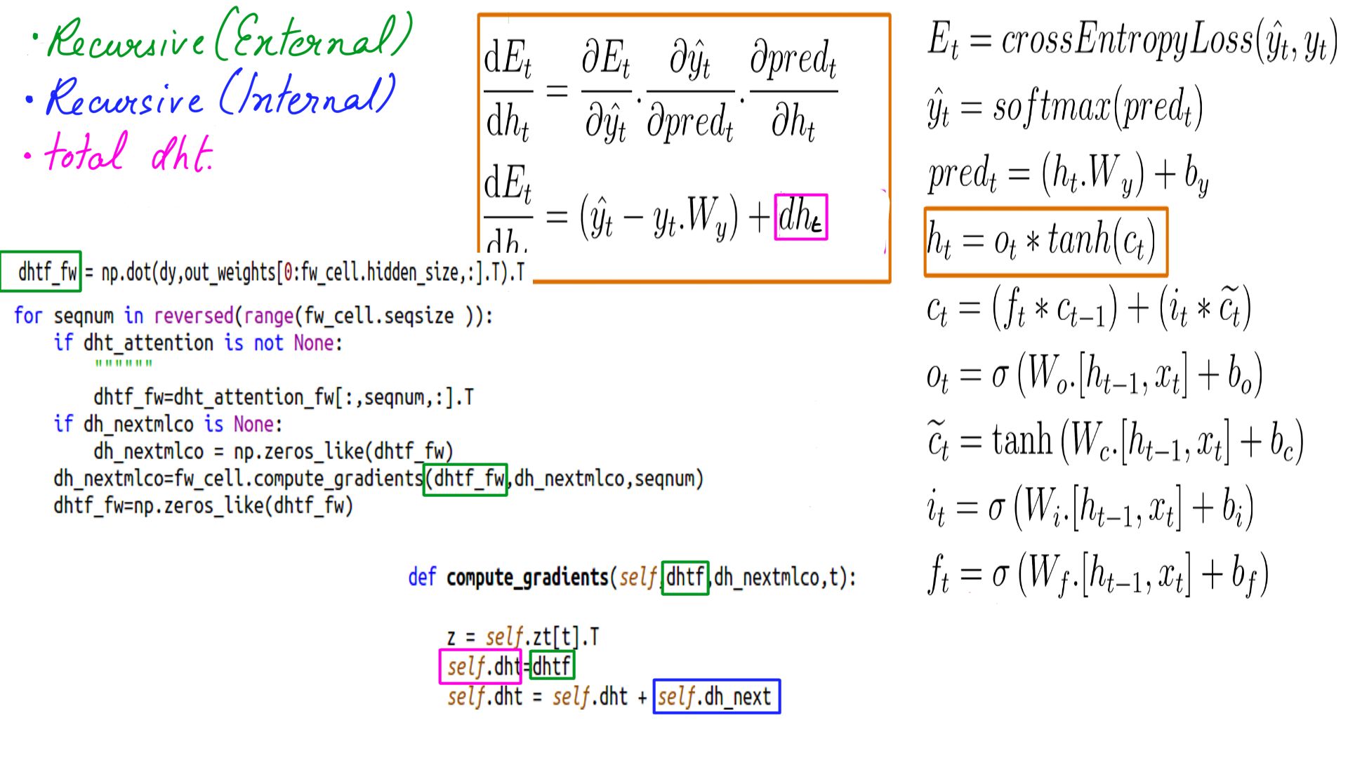
- dHt schematically.Shape is the same as h, for this example it is (5X1)
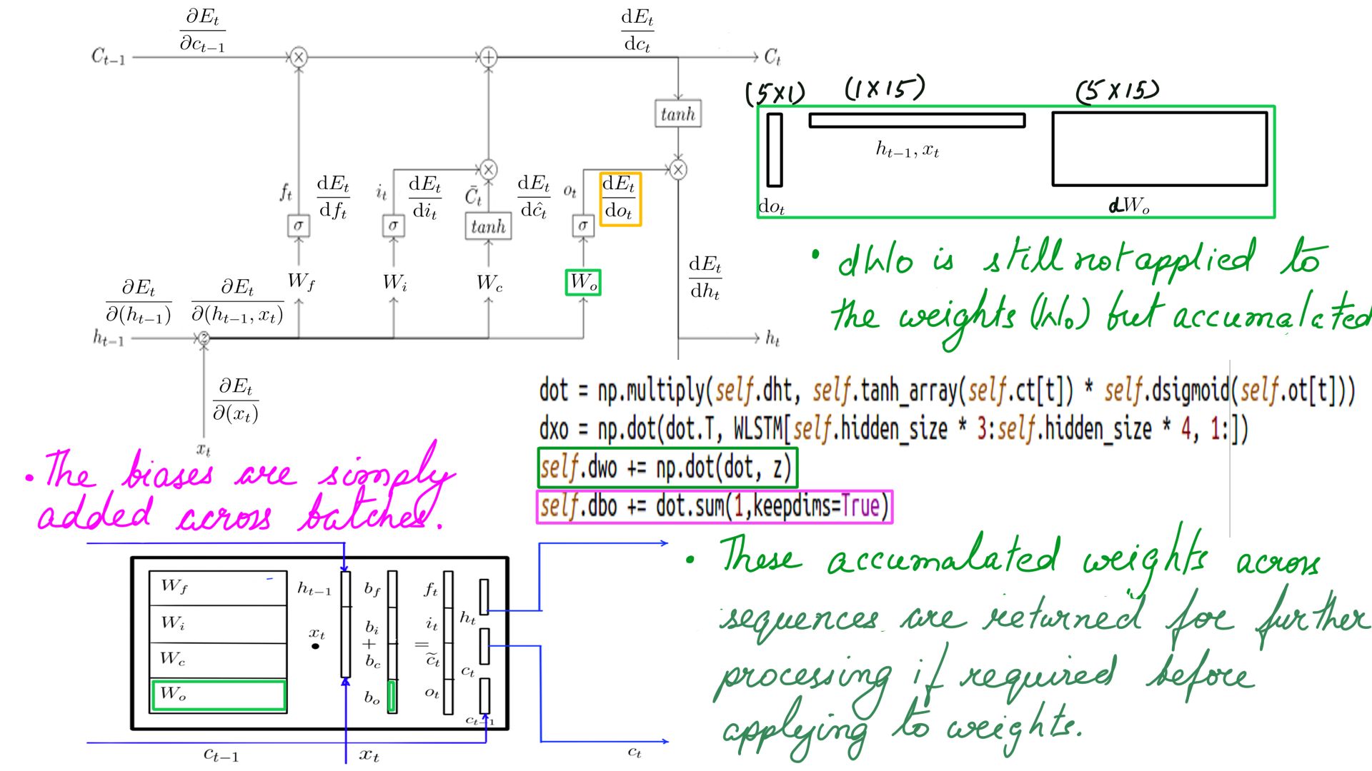
DOt
- Shape of DOt is the same as h, for this example it is (5X1)
- The complete listing is at code-6.

- DOt schematically.
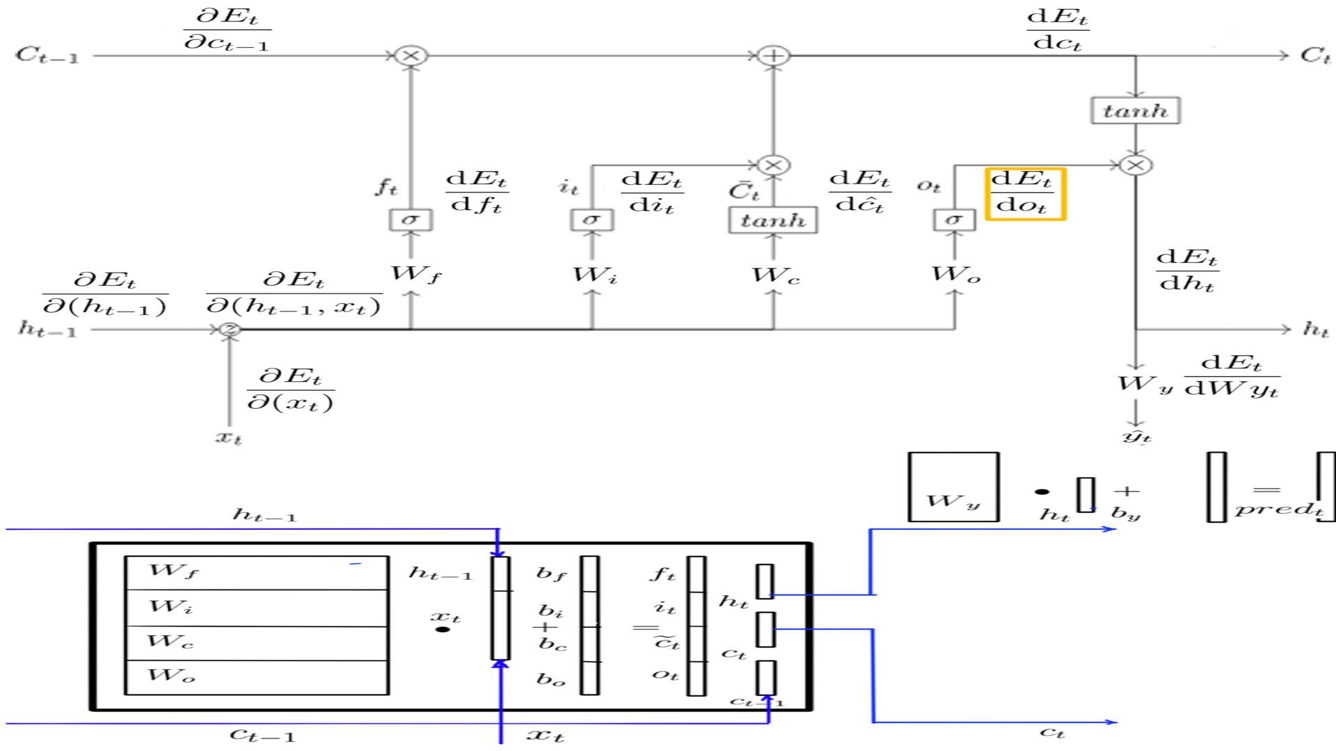
- DOt, DWo and DBo
- Complete listing can be found at code-7
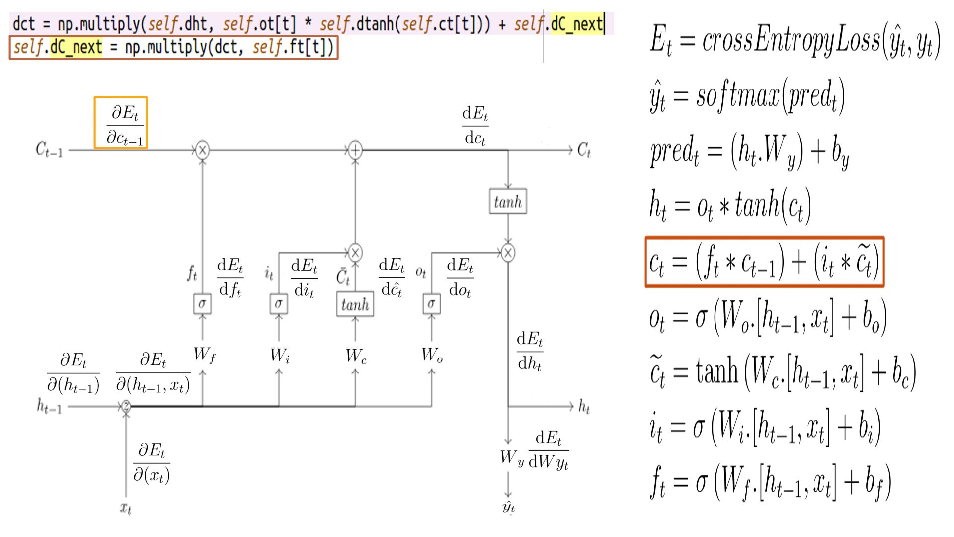
DCt
- Shape of DCt is the same as h, for this example it is (5X1)
- The complete listing is at code-8.
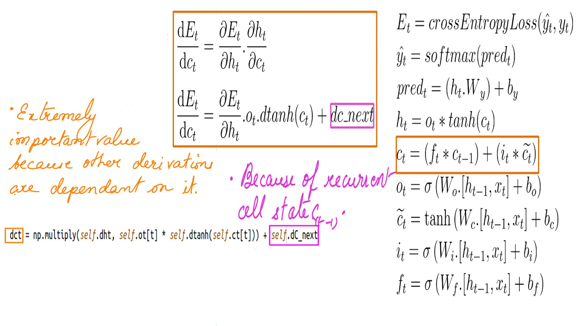
- DCt schematically.
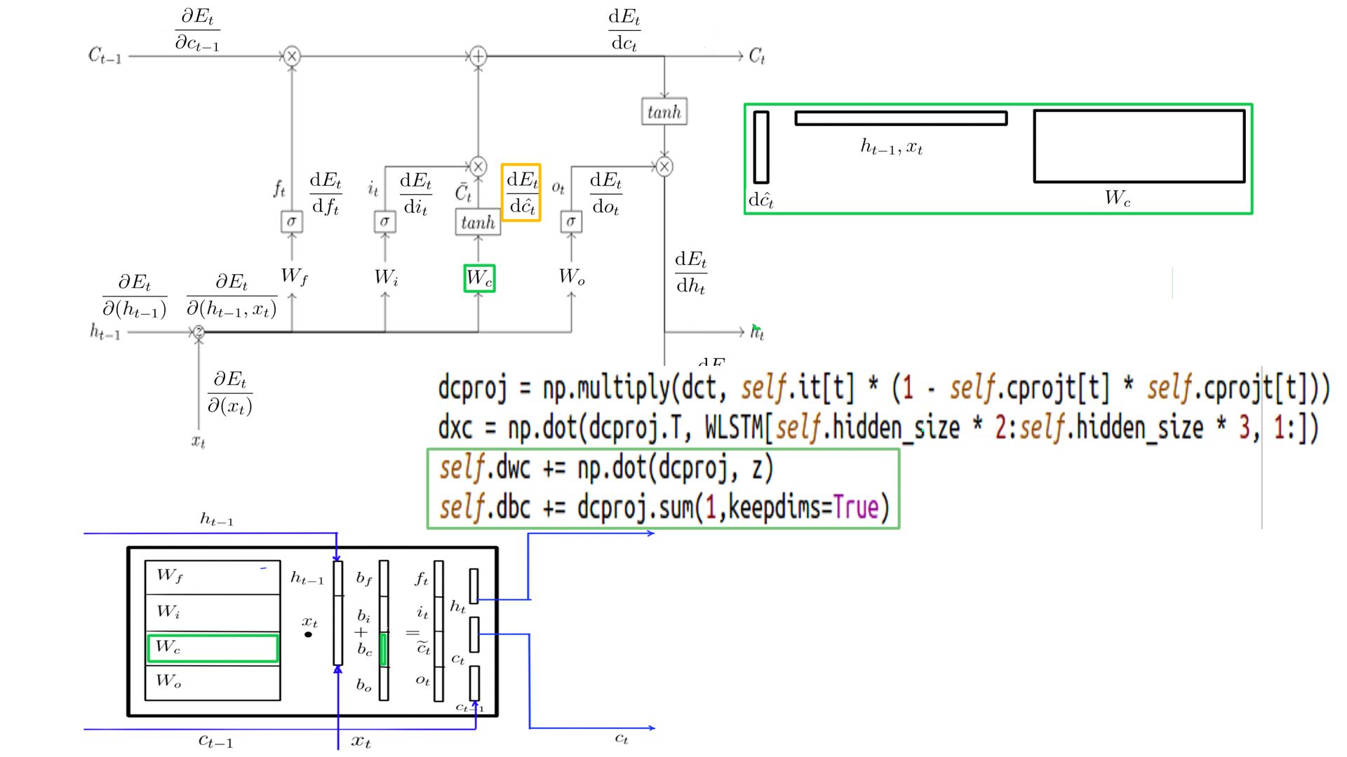
DCprojt
- Shape of DCprojt is the same as h, for this example it is (5X1)
- The complete listing is at code-9.
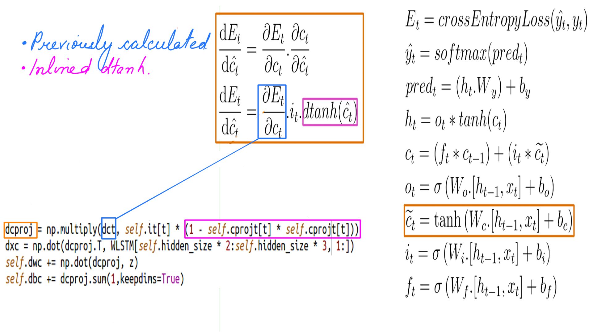
- DCprojt schematically.
- DCprojt
- Complete listing can be found at code-10
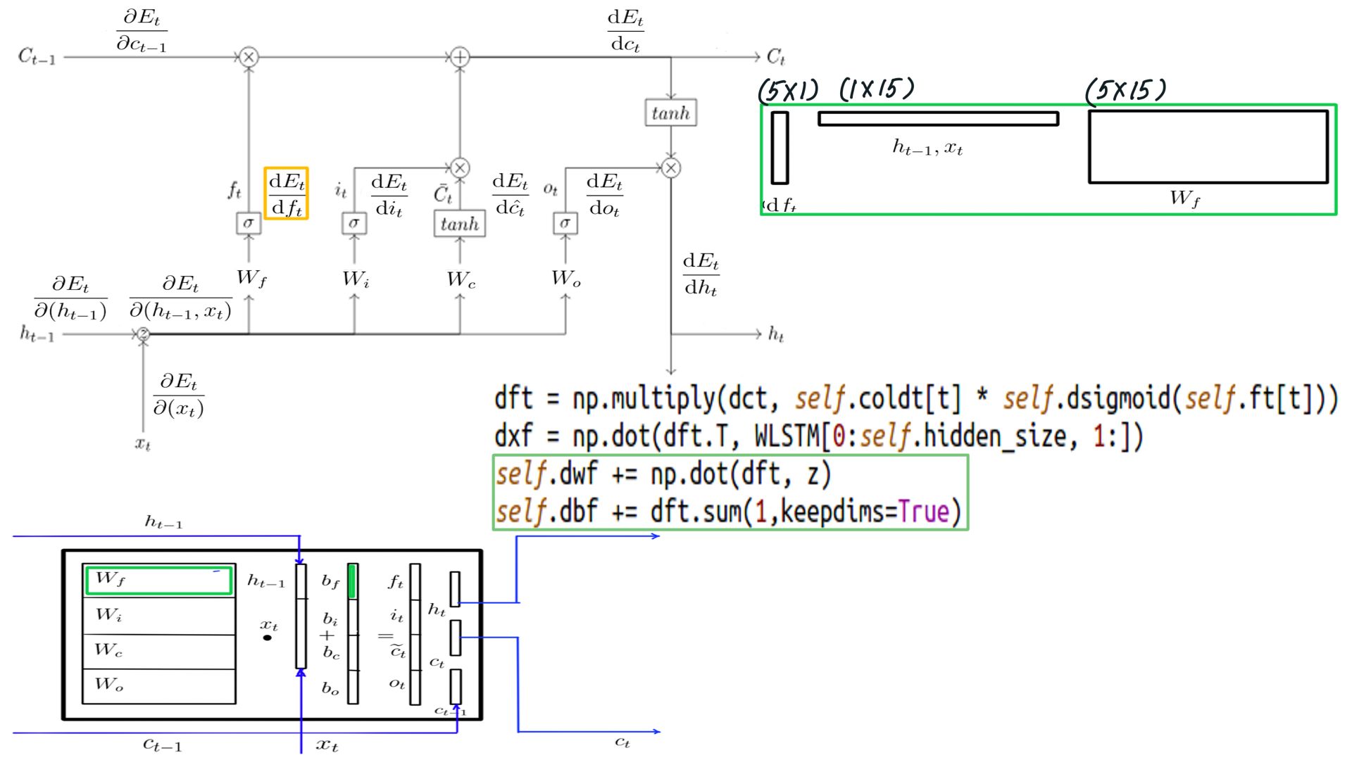
DFt
- Shape of DFt is the same as h, for this example it is (5X1)
- The complete listing is at code-11.
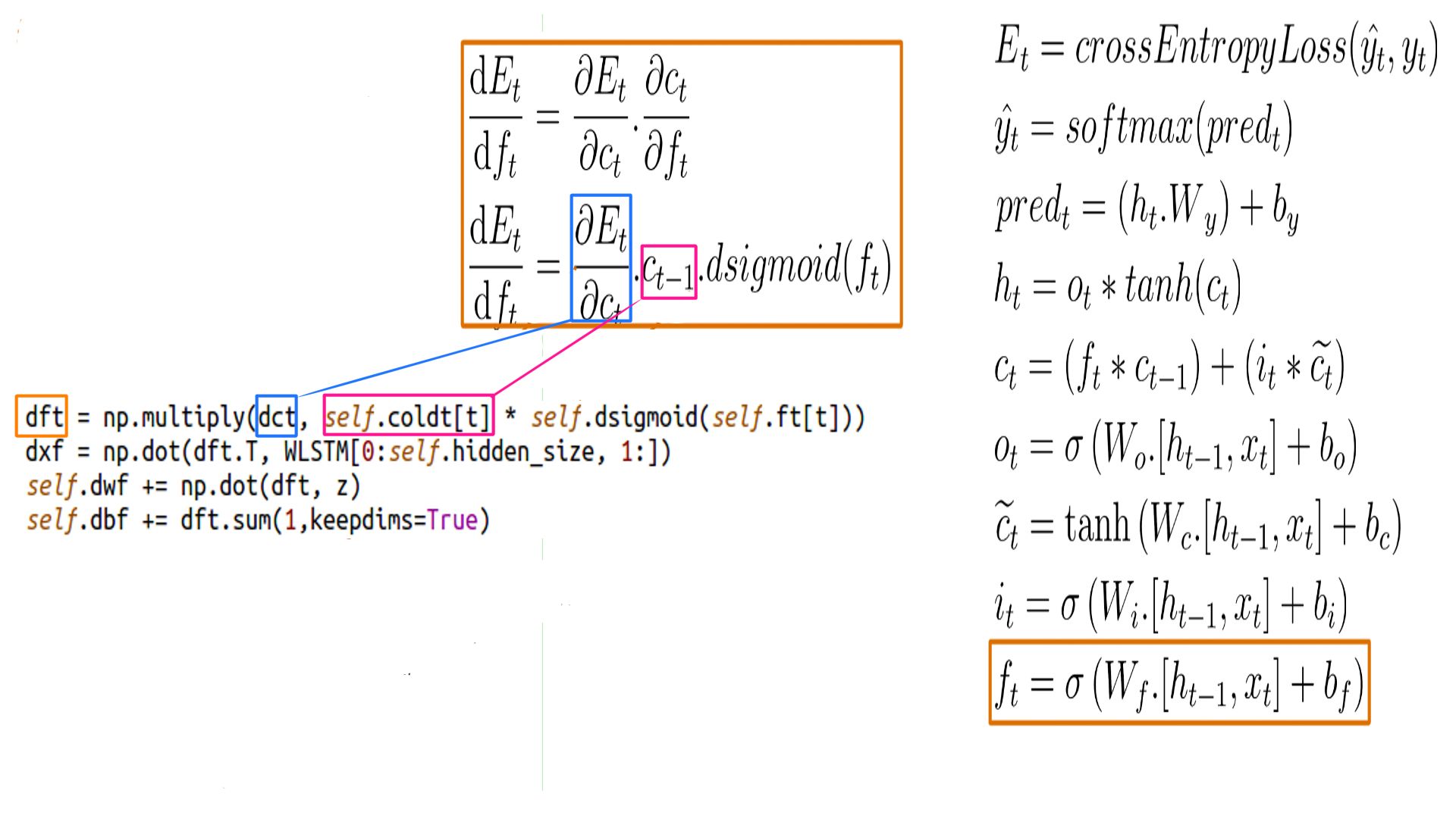
- DFt schematically.
- DFt
- Complete listing can be found at code-12
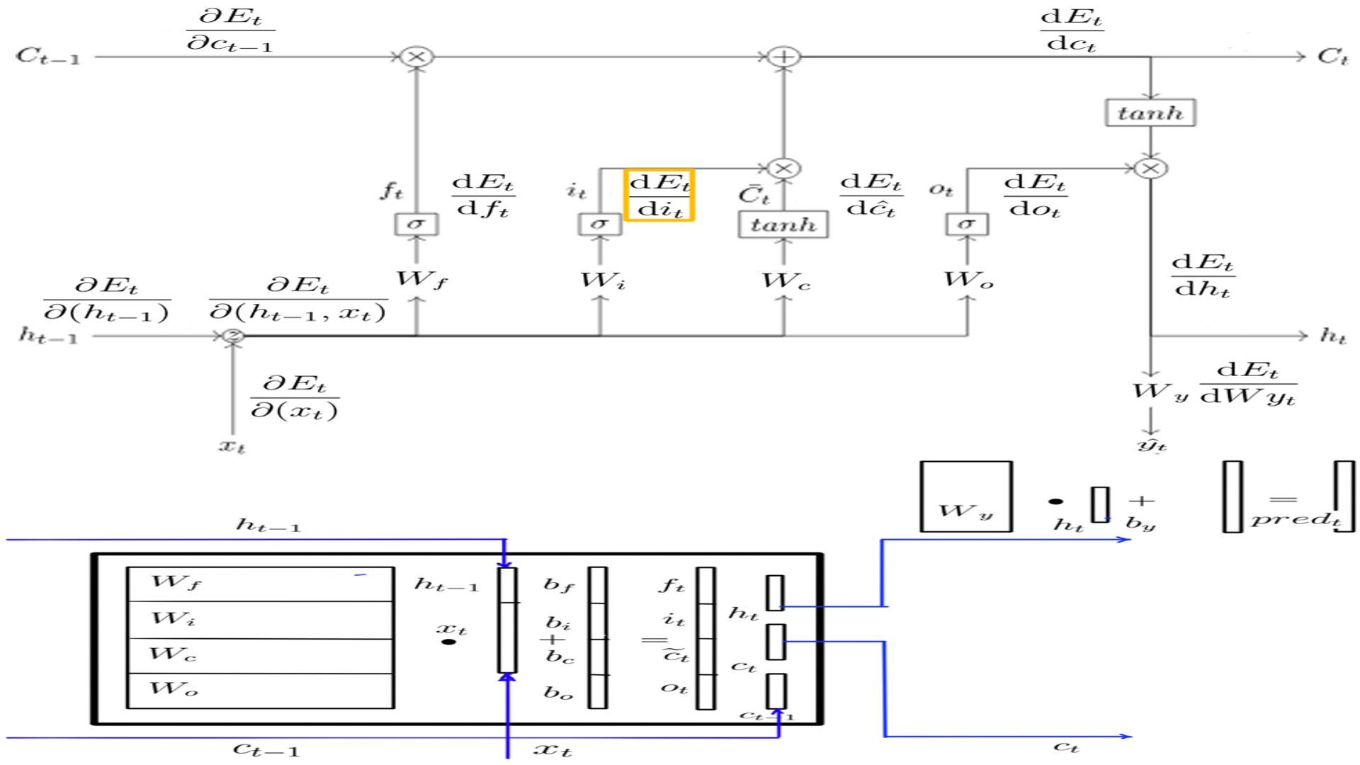
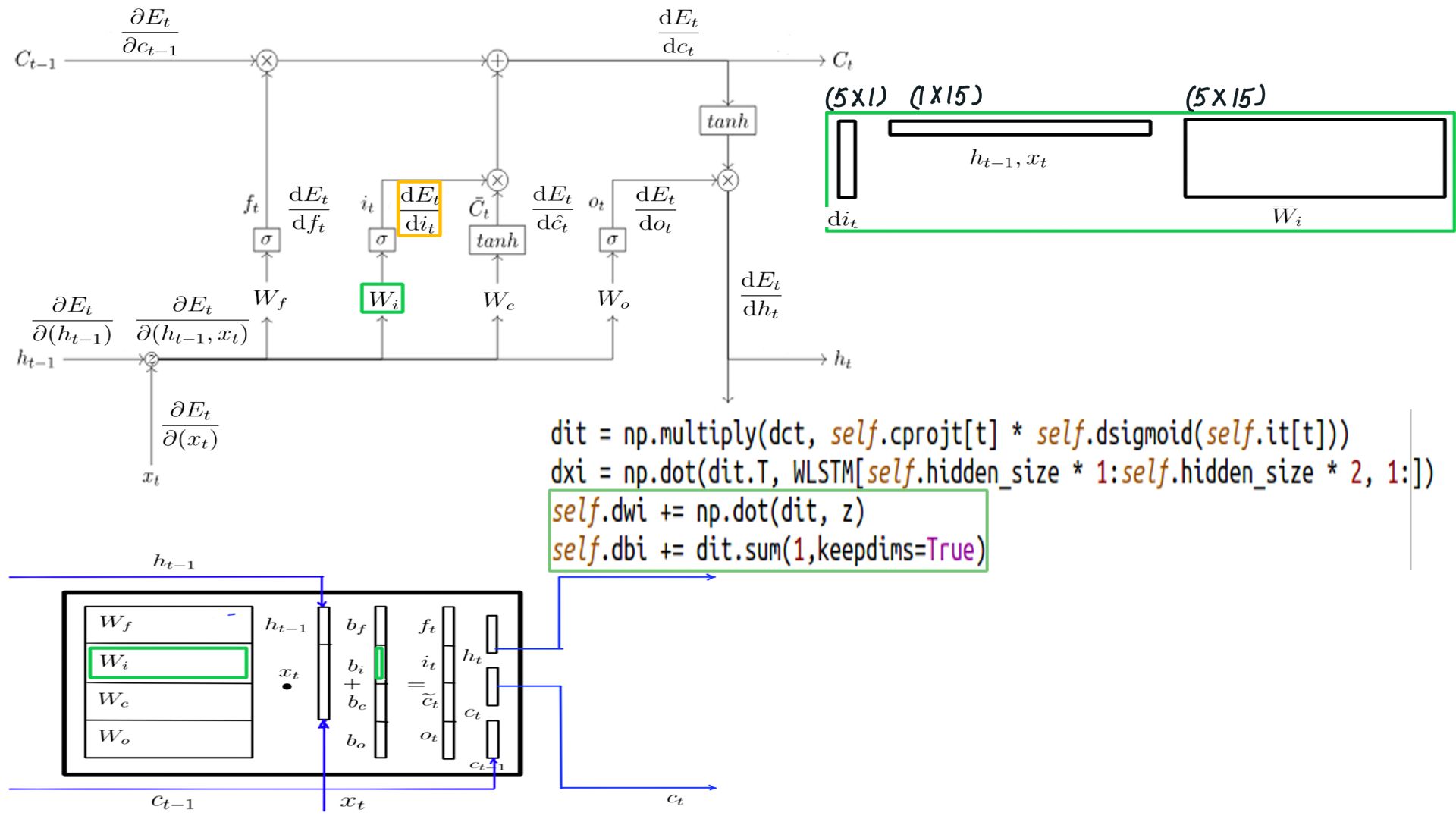
DIt
- Shape of DIt is the same as h, for this example it is (5X1)
- The complete listing is at code-13.
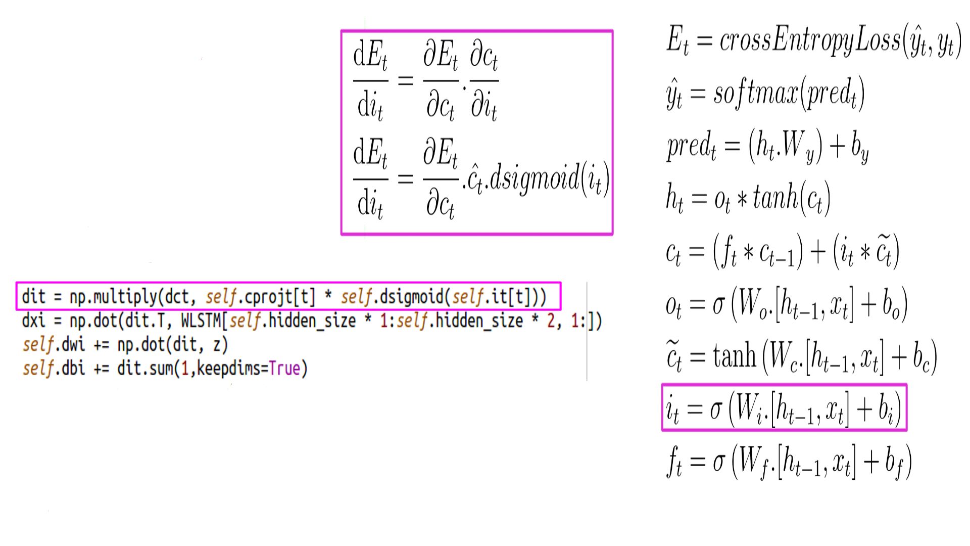
- DIt schematically.
- DIt
- Complete listing can be found at code-14
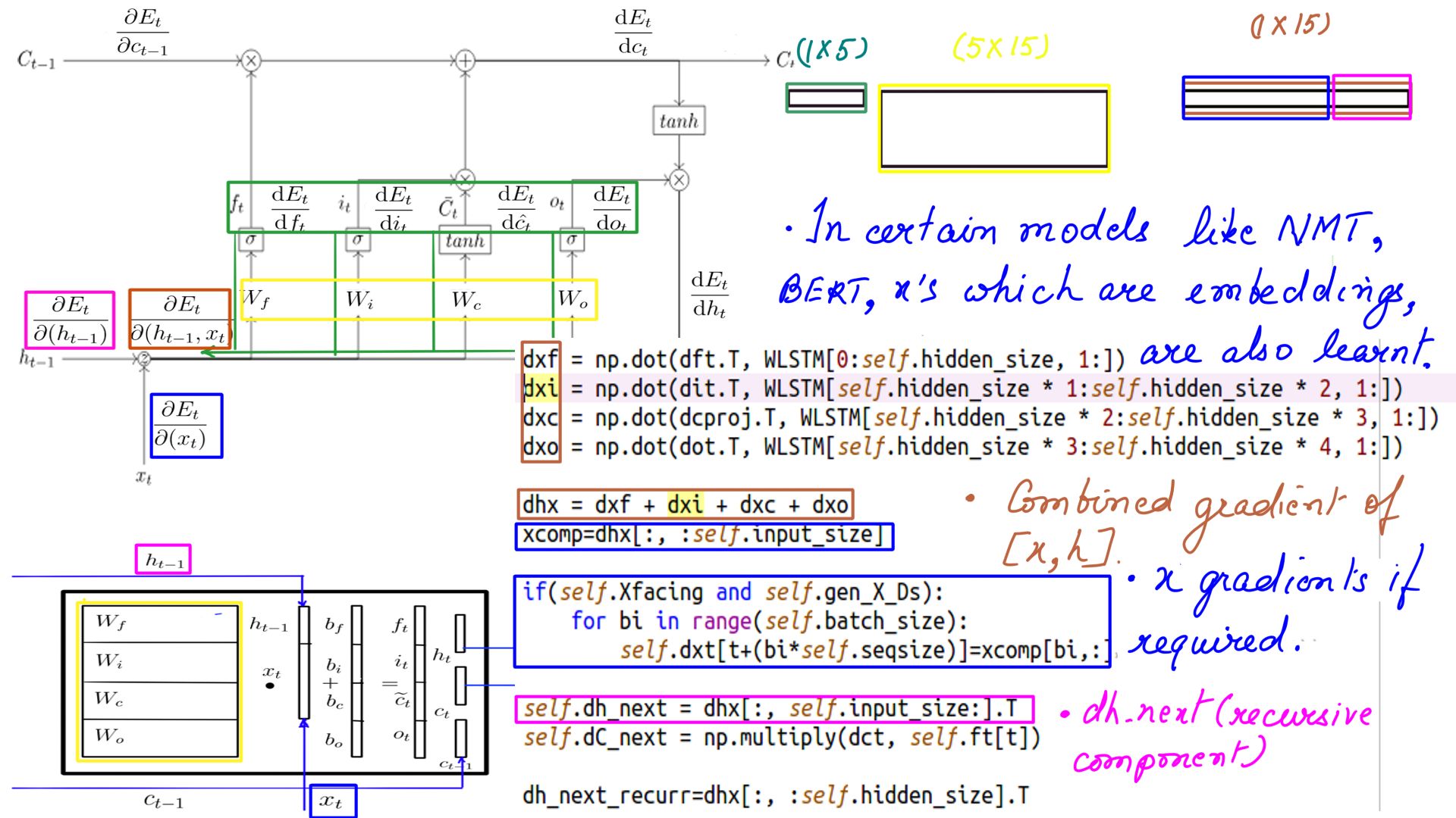
DHX
- Dhx, Dh_next, dxt.
- Complete listing can be found at code-15
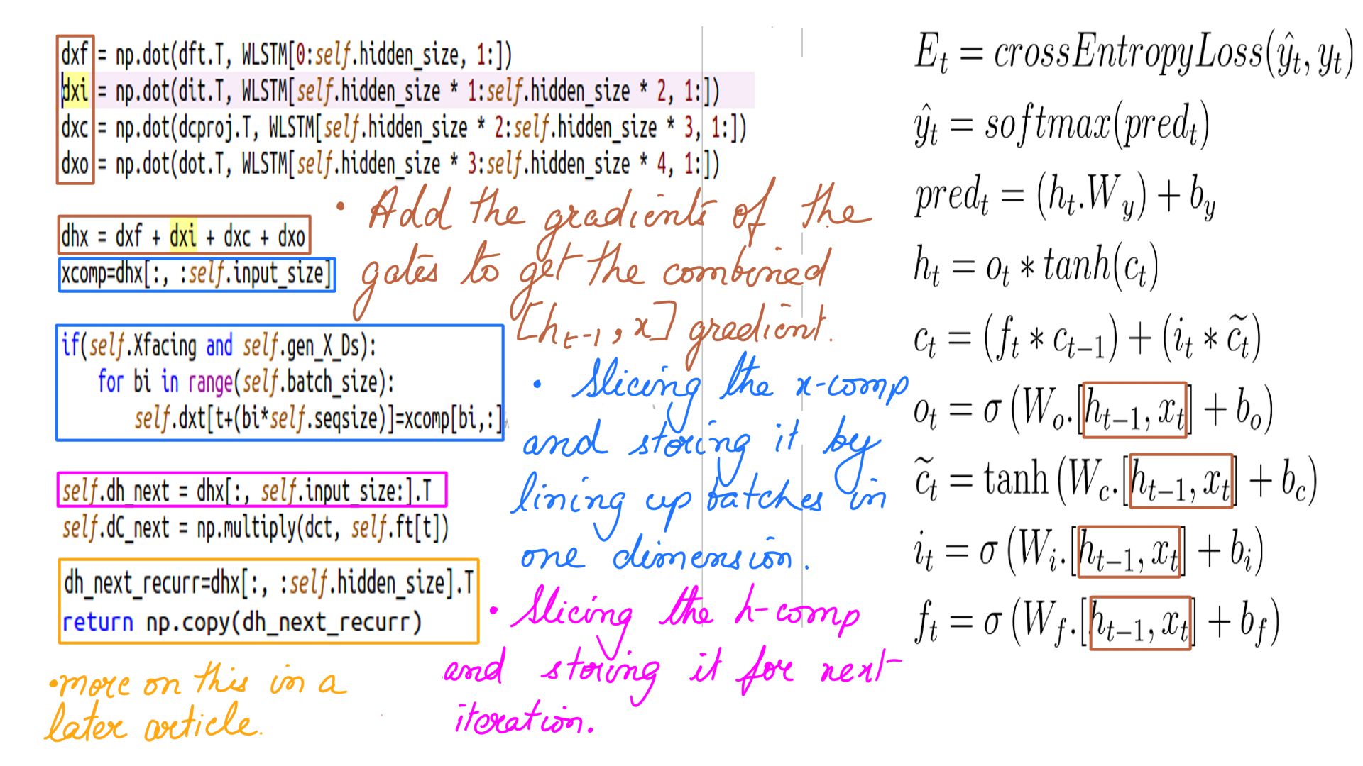
- Many models like Neural Machine Translators(NMT), Bidirectional Encoder Representation from Transformers(BERT) use word embeddings as their inputs(Xs) which oftentimes need learning and that is where we need dxt
DCt_recur
- DCt.
- Complete listing can be found at code-16
Summary
There you go, a complete documentation of LSTMCell’s backward propagation. Also when using Deep-Breathe you could enable forward or backward logging like so
  cell = LSTMCell(n_hidden,debug=False,backpassdebug=True)
  out_l = Dense(10,kernel_initializer=init_ops.Constant(out_weights),bias_initializer=init_ops.Constant(out_biases),backpassdebug=True,debug=False)

  Listing-1
We went through “hell” and back in this article. But if you have come so far then the good news is, it can only get easier. When we do use LSTMs in more complex architecture like Neural Machine Translators(NMT), Bidirectional Encoder Representation from Transformers(BERT), or a Differentiable Neural Computers(DNC) it will be a walk in a blooming lovely park. Well alomost!! ;-). In a later article well demystify the multilayer LSTMcells and Bi-directional LSTMCells.