Softmax and its Gradient

From the perspective of Deep Neural networks, softmax is one the most important activation function, maybe the most important. I had trouble understanding it in the beginning, especially its why its chosen, its gradient, its relationship with cross-entropy loss and the combined gradient. There are many softmax resources available on the internet. Among the many that are available, I found the link here to be the most complete. In this article, I “dumb” it down further and add code to the theory. Code, when associated with theory, makes the explanation very precise. But, there is another selfish reason for reproducing these here, I will be able to refer to these while explaining more complex concepts like LSTMs, NMT, BERT, etc.

Softmax is essentially a vector function. It takes n inputs and produces and n outputs. The out can be interpreted as a probabilistic output(summing up to 1). A multiway shootout if you will.

And the actual per-element formula is:

As one can see the output function can only be positive because of the exponential and the values range between 0 and 1. Also, the value appears in the denominator summed up with other positive numbers.

def softmax(logits):
    #row represents num classes but they may be real numbers
    #So the shape of input is important
    #([[1, 3, 5, 7],
    #  [1,-9, 4, 8]]

    #softmax will be for each of the 2 rows
    #[[2.14400878e-03 1.58422012e-02 1.17058913e-01 8.64954877e-01]
    #[8.94679461e-04 4.06183847e-08 1.79701173e-02 9.81135163e-01]]
    #respectively But if the input is Tranposed clearly the answer
    #will be wrong.

    #That needs to be converted to probability
    #column represents the vocabulary size.

    r, c = logits.shape
    predsl = []
    for row in logits:
        inputs = np.asarray(row)
        #print("inputs:",inputs)
        predsl.append(np.exp(inputs) / float(sum(np.exp(inputs))))
    return np.array(predsl)

Above is a softmax implementation.

    x = np.array([[1, 3, 5, 7],
          [1,-9, 4, 8]])
    print("x:",x)
    sm=softmax(x)
    print("softmax:",sm)
    #prints out
    #[[2.14400878e-03 1.58422012e-02 1.17058913e-01 8.64954877e-01],
    #[8.94679461e-04 4.06183847e-08 1.79701173e-02 9.81135163e-01]]

Above is a softmaxtest implementation.

The softmax function is very similar to the Logistic regression cost function. The only difference being that the sigmoid makes the output binary interpretable whereas, softmax’s output can be interpreted as a multiway shootout. With the above two rows individually summing up to one.

Softmax Derivative

Before diving into computing the derivative of softmax, let’s start with some preliminaries from vector calculus.

Softmax is fundamentally a vector function. It takes a vector as input and produces a vector as output; in other words, it has multiple inputs and multiple outputs. Therefore, we cannot just ask for “the derivative of softmax”; We should instead specify:

1. Which component (output element) of softmax we’re seeking to find the derivative of.
2. Since softmax has multiple inputs, with respect to which input element the partial derivative is being computed. This is exactly why the notation of vector calculus was developed. What we’re looking for is the partial derivatives:

This is the partial derivative of the i-th output w.r.t. the j-th input. A shorter way to write it that we’ll be using going forward is: Since softmax is a function, the most general derivative we compute for it is the Jacobian matrix:

Let’s compute \(D_jsoftmax_i\) for arbitrary i and j:

\(\large D_jsoftmax_i=\Large \:\:\frac{\partial softmax_i}{\partial a_j}\:\:= \frac{\partial \frac{e^{a_j}}{\sum_{k=1}^{N} e^{a_k}}}{\partial a_j}\)
Using the quotient rule \(\Large f(x) = \frac{g(x)}{h(x)}\) , \(\Large f'(x) = \frac{g'(x)h(x) - h'(x)g(x)}{h(x)^2}\)
in our case \(\Large g_i = e^{a_i}\)
                   \(\Large h_i = \sum_{k=1}^{N} e^{a_k}\) simplifying \(\Large \sum\) for \(\Large \sum_{k=1}^{N} e^{a_k}\)

Note that no matter which \(a_j\) we compute the derivative of \(h_i\) for, the answer will always be \(e^{a_j}\). This is not the case for \(g_i\), howewer. The derivative of \(g_i\) w.r.t. \(a_j\) is \(e^{a_j}\) only if i=j, because only then \(g_i\) has \(a_j\) anywhere in it. Otherwise, the derivative is 0.

1. Going back to our \(\Large \frac{\partial softmax_i}{\partial a_j}\) we’ll start with the \(\Large i=j\) case.
   Then, using the quotient rule we have: \(\Large \frac{\partial\frac{e^{a_j}}{\sum_{k=1}^{N} e^{a_k}}}{\partial a_j} = \frac{e^{a_i}.\sum-e^{a_j}.e^{a_i}}{\sum^2}\)
                            \(\Large = \frac{e^{a_i}}{\sum}.\frac{\sum-e^{a_j}}{\sum}\)
                            \(\Large = softmax_i(1-softmax_j)\)

2. similarly for \(\Large i \neq j\)
   \(\Large \frac{\partial\frac{e^{a_j}}{\sum_{k=1}^{N} e^{a_k}}}{\partial a_j} = \frac{0- e^{a_j}e^{a_i}}{\sum^2}\)
                            \(\Large = \frac{- e^{a_j}}{\sum}.\frac{e^{a_i}}{\sum}\)
                            \(\Large = {-softmax_j}.{softmax_i}\)

To summarize:
\(\Large D_jsoftmax_i=\begin{Bmatrix} softmax_i(1-softmax_j) & i= j \\ {-softmax_j}.{softmax_i} & i\neq j \end{Bmatrix} \:\:\:\: eq(1)\)

Softmax Derivative Implementation

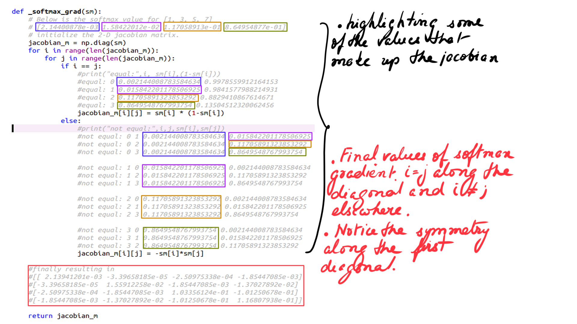
def _softmax_grad(sm):
    # Below is the softmax value for [1, 3, 5, 7]
    # [2.14400878e-03 1.58422012e-02 1.17058913e-01 8.64954877e-01]
    # initialize the 2-D jacobian matrix.
    jacobian_m = np.diag(sm)
    for i in range(len(jacobian_m)):
        for j in range(len(jacobian_m)):
            if i == j:
                print("equal:",i, sm[i],(1-sm[i]))
                #equal: 0 0.002144008783584634 0.9978559912164153
                #equal: 1 0.015842201178506925 0.9841577988214931
                #equal: 2 0.11705891323853292 0.8829410867614671
                #equal: 3 0.8649548767993754 0.13504512320062456
                jacobian_m[i][j] = sm[i] * (1-sm[i])
            else:
                print("not equal:",i,j,sm[i],sm[j])
                #not equal: 0 1 0.002144008783584634 0.015842201178506925
                #not equal: 0 2 0.002144008783584634 0.11705891323853292
                #not equal: 0 3 0.002144008783584634 0.8649548767993754

                #not equal: 1 0 0.015842201178506925 0.002144008783584634
                #not equal: 1 2 0.015842201178506925 0.11705891323853292
                #not equal: 1 3 0.015842201178506925 0.8649548767993754

                #not equal: 2 0 0.11705891323853292 0.002144008783584634
                #not equal: 2 1 0.11705891323853292 0.015842201178506925
                #not equal: 2 3 0.11705891323853292 0.8649548767993754

                #not equal: 3 0 0.8649548767993754 0.002144008783584634
                #not equal: 3 1 0.8649548767993754 0.015842201178506925
                #not equal: 3 2 0.8649548767993754 0.11705891323853292
                jacobian_m[i][j] = -sm[i]*sm[j]

    #finally resulting in
    #[[ 2.13941201e-03 -3.39658185e-05 -2.50975338e-04 -1.85447085e-03]
    #[-3.39658185e-05  1.55912258e-02 -1.85447085e-03 -1.37027892e-02]
    #[-2.50975338e-04 -1.85447085e-03  1.03356124e-01 -1.01250678e-01]
    #[-1.85447085e-03 -1.37027892e-02 -1.01250678e-01  1.16807938e-01]]

    return jacobian_m

The above is the softmax grad code. As you can see it initializes a diagonal matrix that is then populated with the right values. On the main diagonal it has the values for case (i=j) and (i!=j) elsewhere. This is illustrated in the picture below.

Summary

As you can see the softmax gradient producers an nxn matrix for input size of n. Hopefully, you got a good idea of softmax and its implementation. Hopefully, you got a good idea of softmax’s gradient and its implementation. Softmax is usually used along with cross_entropy_loss, but not always. There are few a instances like “Attention”. More on Attention in a much later article. But for now, what is the relationship between softmax and cross_entropy_loss function. This will be illustrated in the next article.