Introduction
In this multi-part series, we look inside LSTM forward pass. If you haven’t already read it I suggest run through the previous parts (part-1) before you come back here. Once you are back, in this article, we explore the meaning, math and the implementation of an LSTM cell. I do this using the first principles approach for which I have pure python implementation Deep-Breathe of most complex Deep Learning models.
What this article is not about?
- This article will not talk about the conceptual model of LSTM, on which there is some great existing material here and here in the order of difficulty.
- This is not about the differences between vanilla RNN and LSTMs, on which there is an awesome post by Andrej if a somewhat difficult post.
- This is not about how LSTMs mitigate the vanishing gradient problem, on which there is a little mathy but awesome posts here and here in the order of difficulty
What this article is about?
- Using the first principles we picturize/visualize the forward pass of an LSTM cell.
- Then we associate code with the picture to make our understanding more concrete
Context
This is the same example and the context is the same as described in part-1. The focus however, this time is on LSTMCell.
LSTM Cell
While there are many variations to the LSTM cell. In the current article, we are looking at LayerNormBasicLSTMCell.
- Weights and biases of the LSTM cell.
- Shapes color-coded.
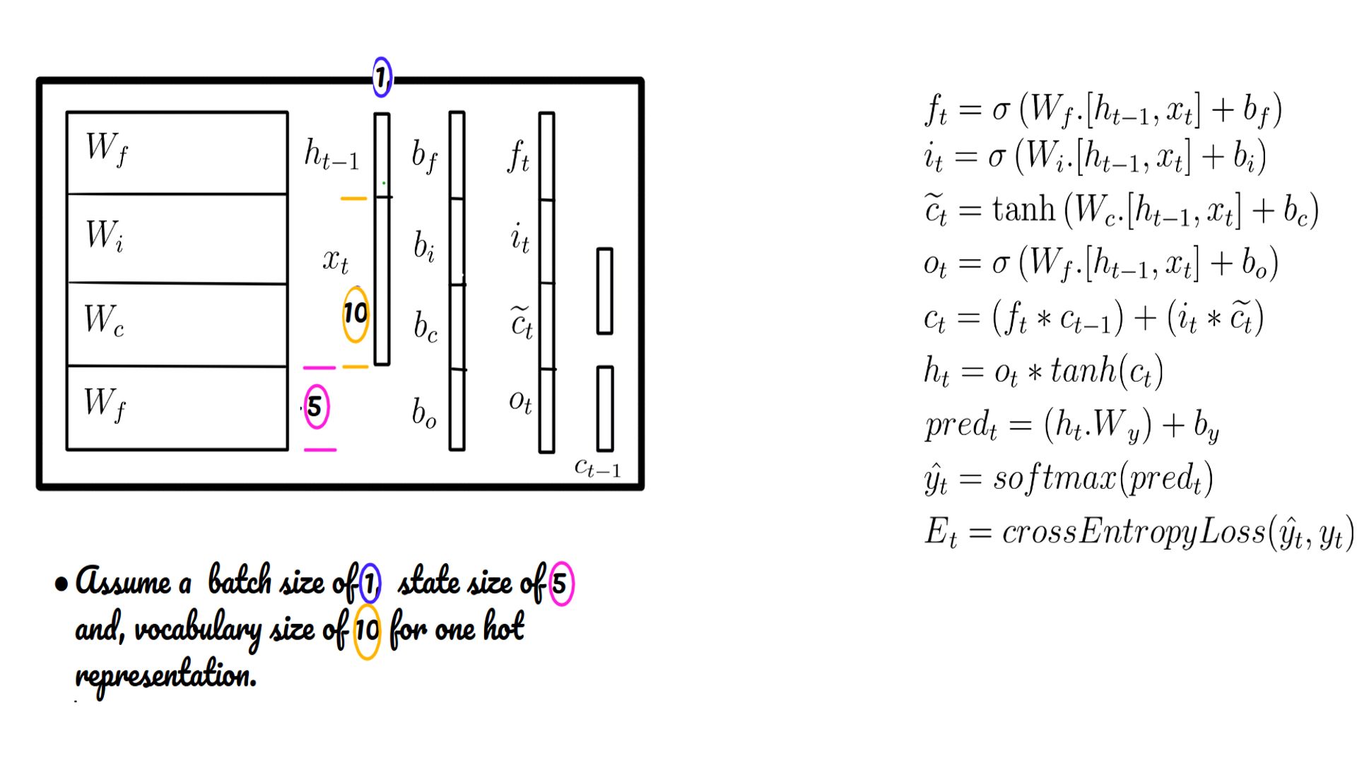
- Weights, biases of the LSTM cell. Also shown is the cell state (c-state) over and above the h-state of a vanilla RNN.
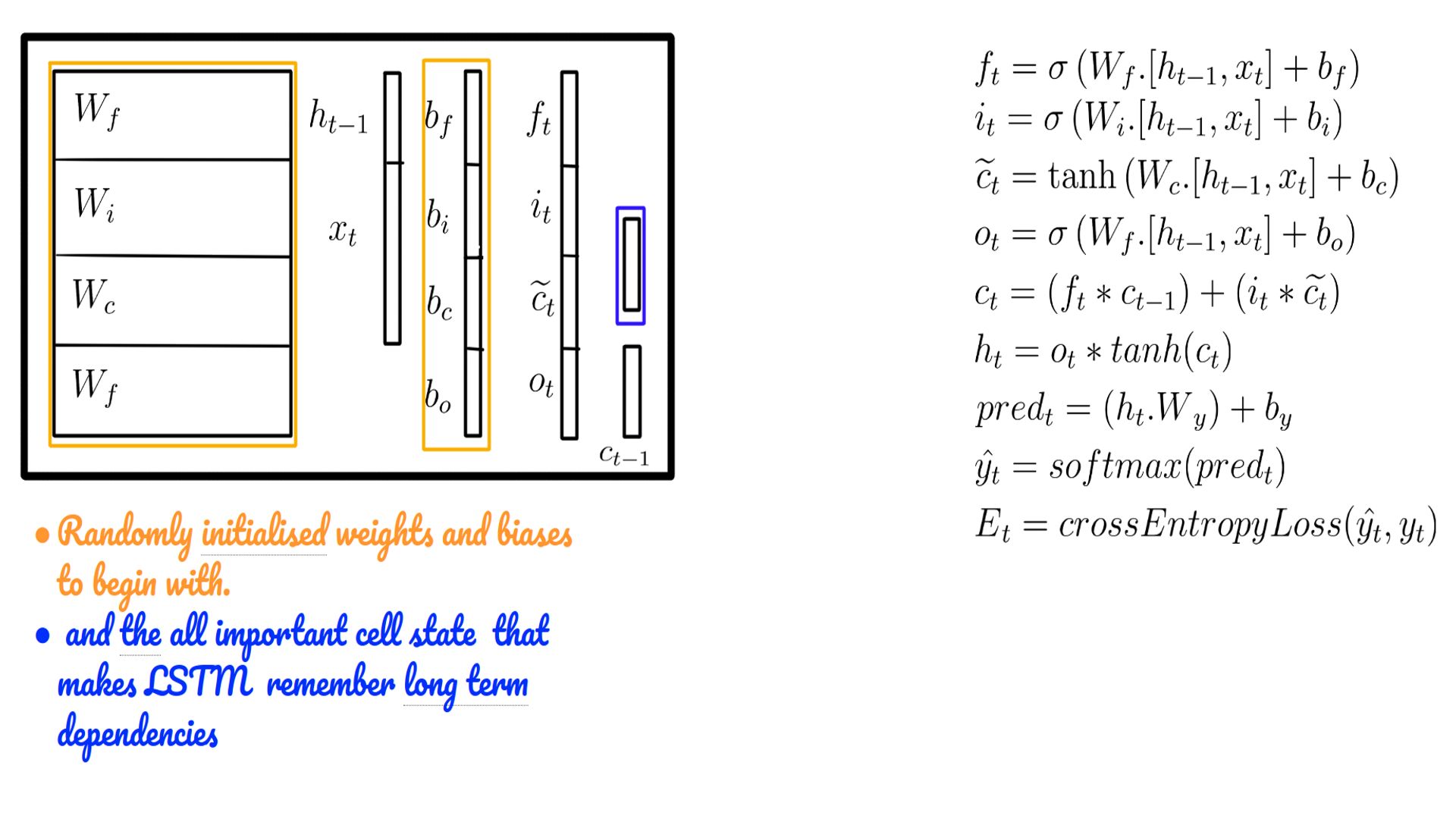
- ht-1 may be initialized by default with zeros.
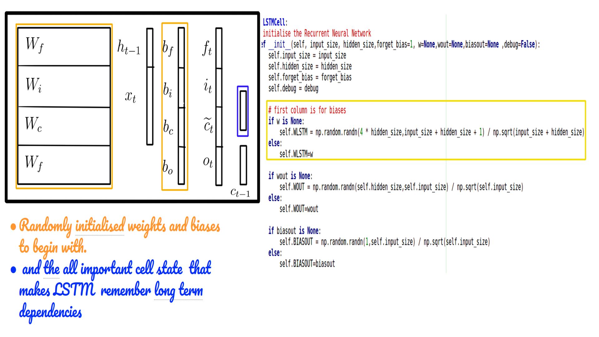
- Weights and biases in the code.
- Often the code accepts constants as weights for comparison with Tensorflow
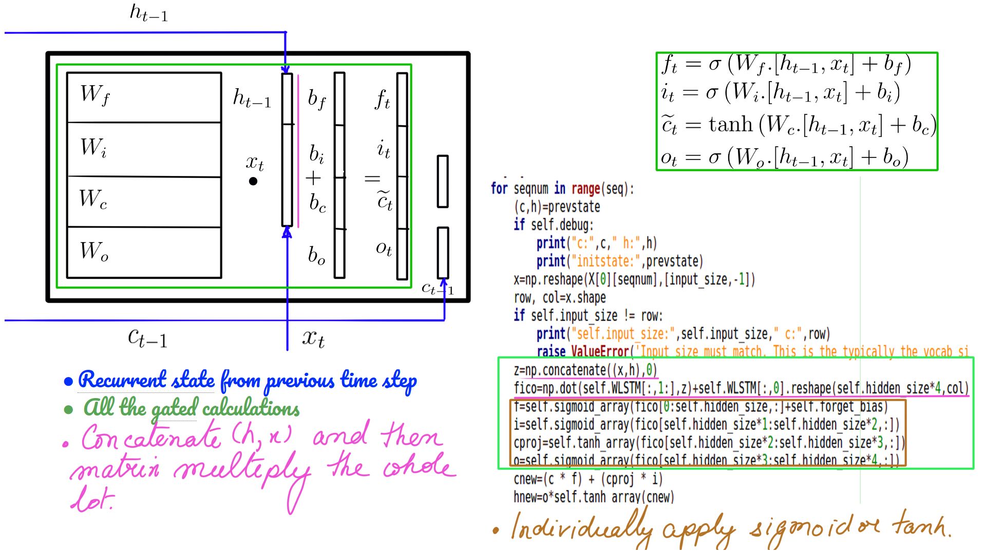
- Equations of LSTM and their interplay with weights and biases.
- ht-1 and ct-1 may be initialized by default with zeros(Language Model) or some non-zero state for conditional language model.
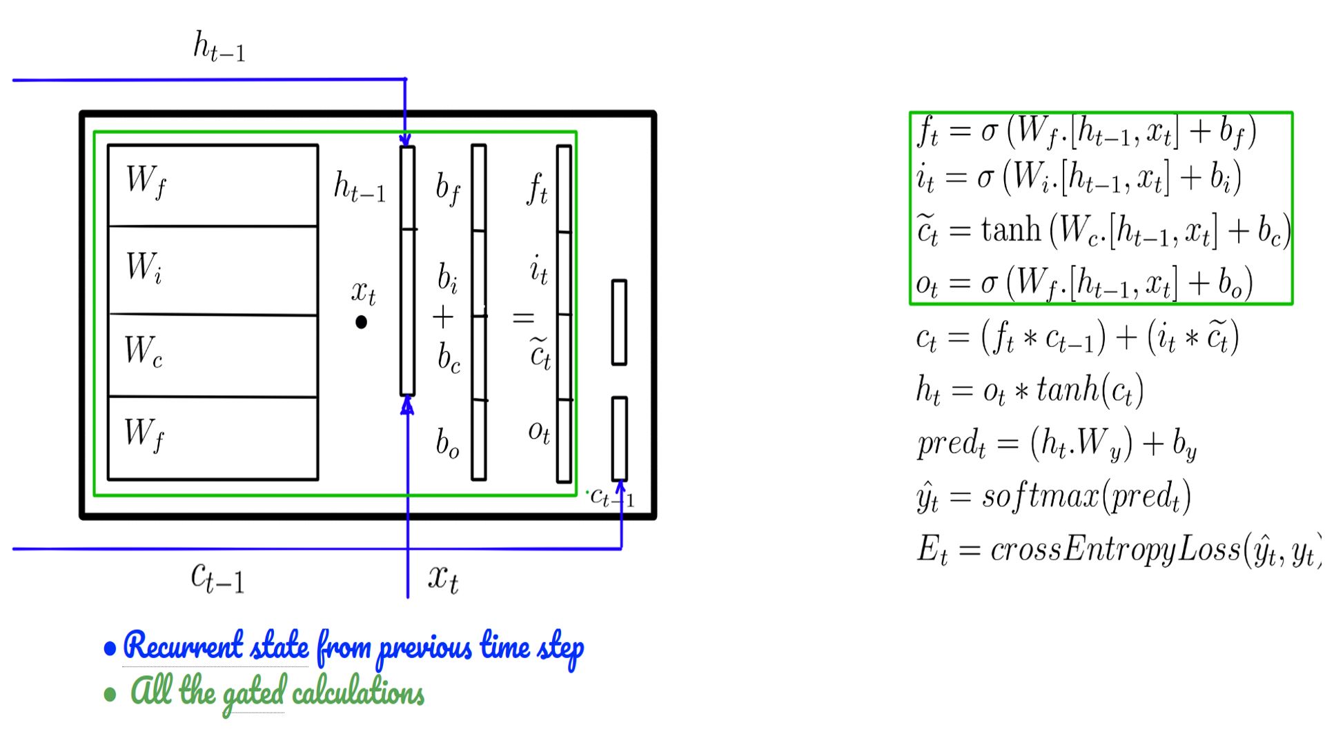
- GEMM(General Matrix Multiplication) in code
- h and x concatenation is only a performance convenience.
- The mathematical reason why the vanishing gradient is mitigated.
- There are many theories though. Look into this in detail with back-propagation.
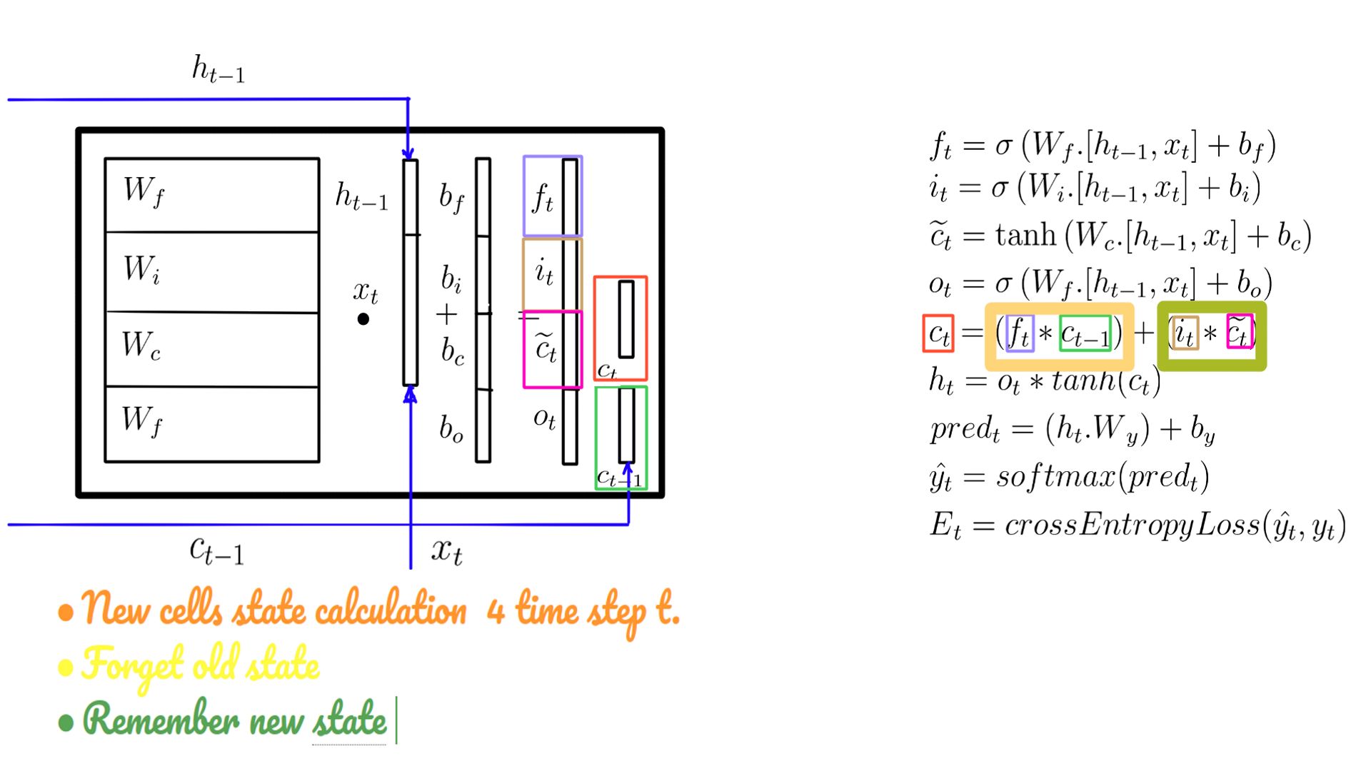
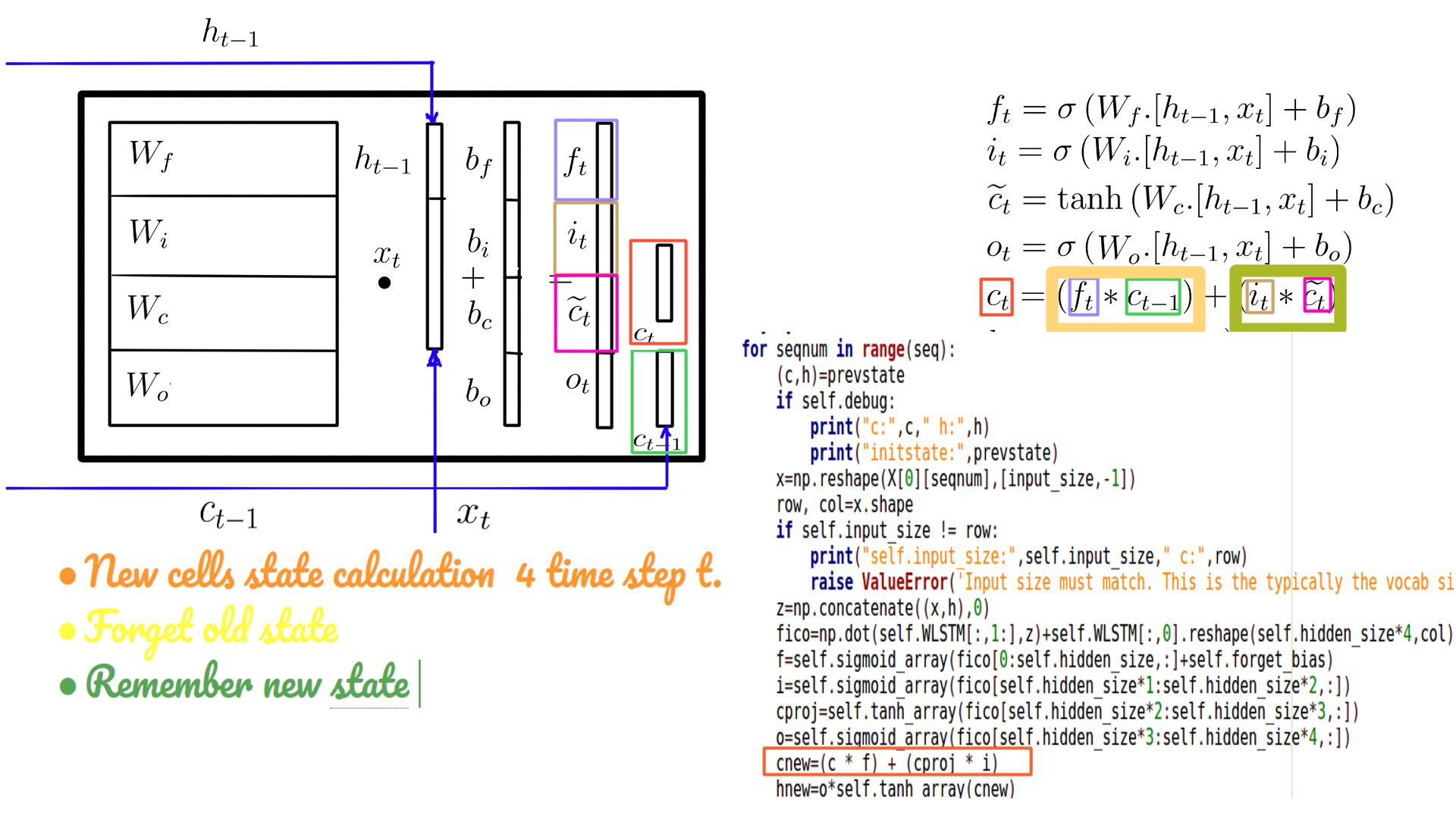
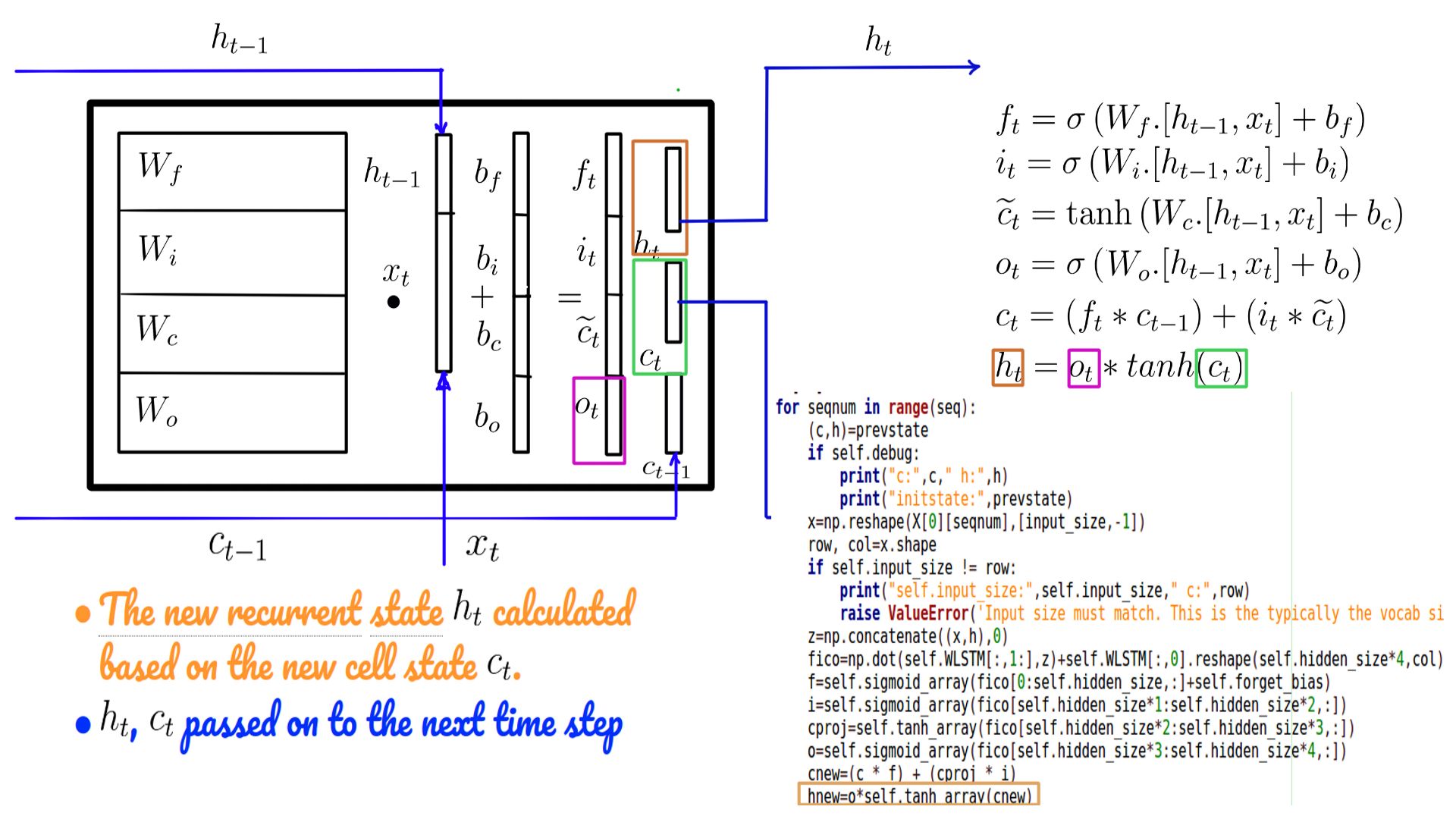
- New cell state(c-state) in code
- This is used in 2 ways as illustrated in figure-8.
- c-statet is used to calculate the “externally visible” h-statet
- Sometimes referred to as ct, ht, used as the states at the next time step.
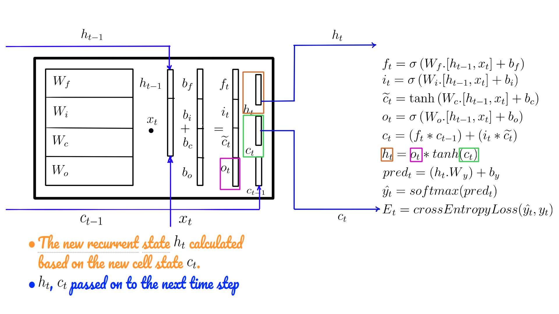
- New h-state in code
- The transition to the next time step is complete with ht.
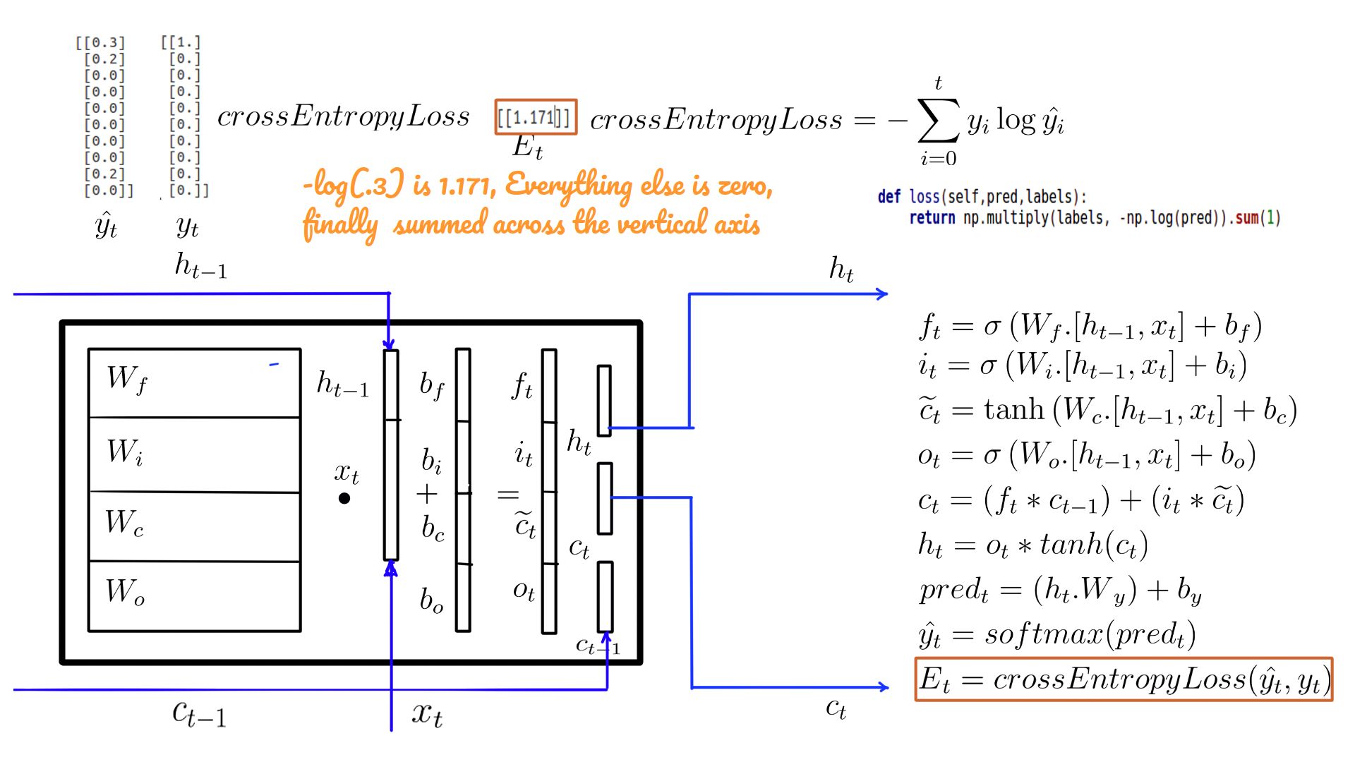
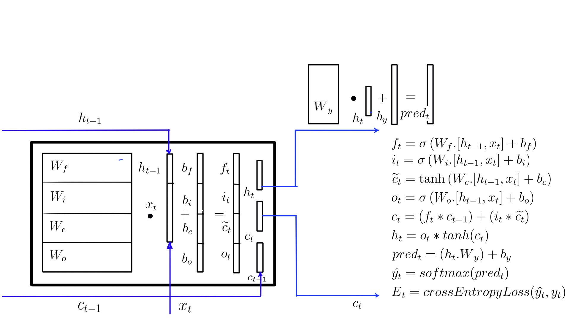
- ht multiplied by the “Wy” and “by” added to it.
- Traditionally we call this value “logits” or “preds”.
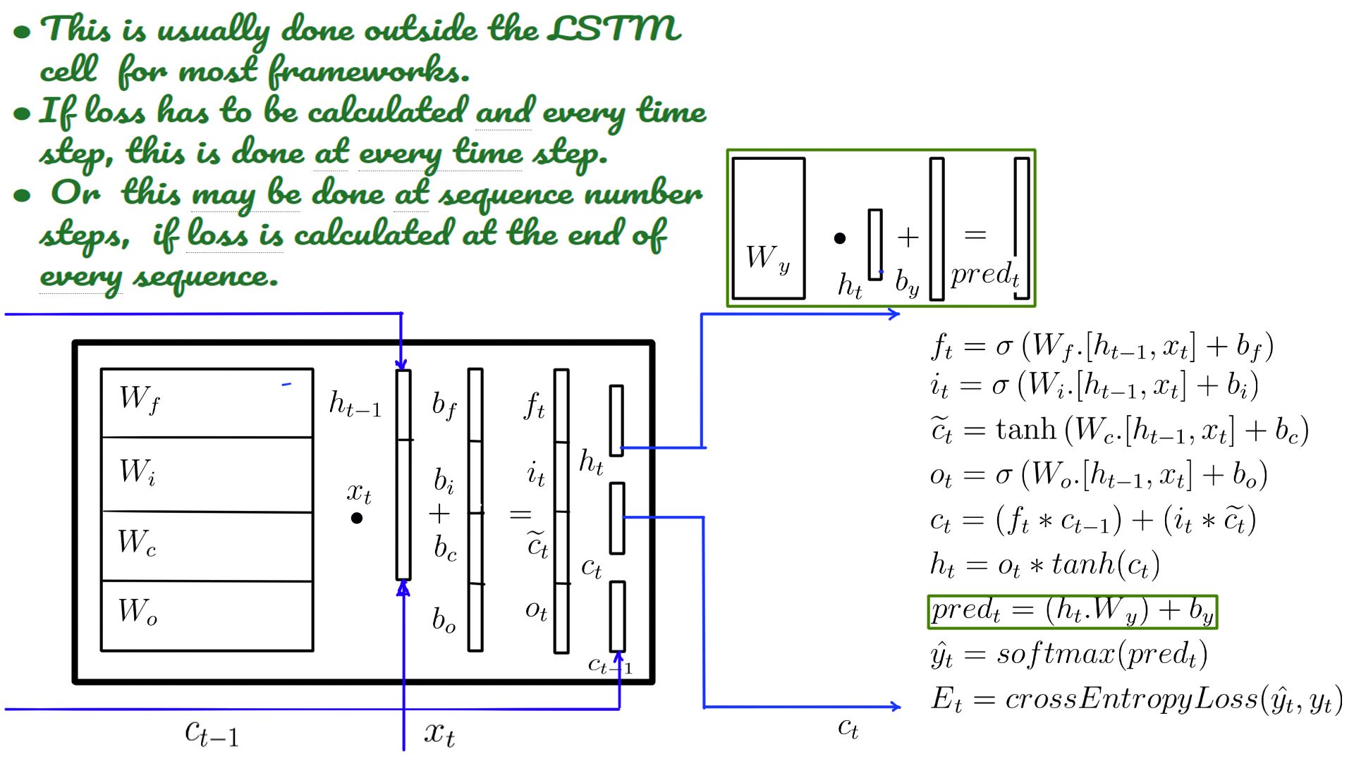
- Usually, this is done in on the client-side code because only the clients know the model and when the loss calculation can be done.
- Tensorflow version of the code.
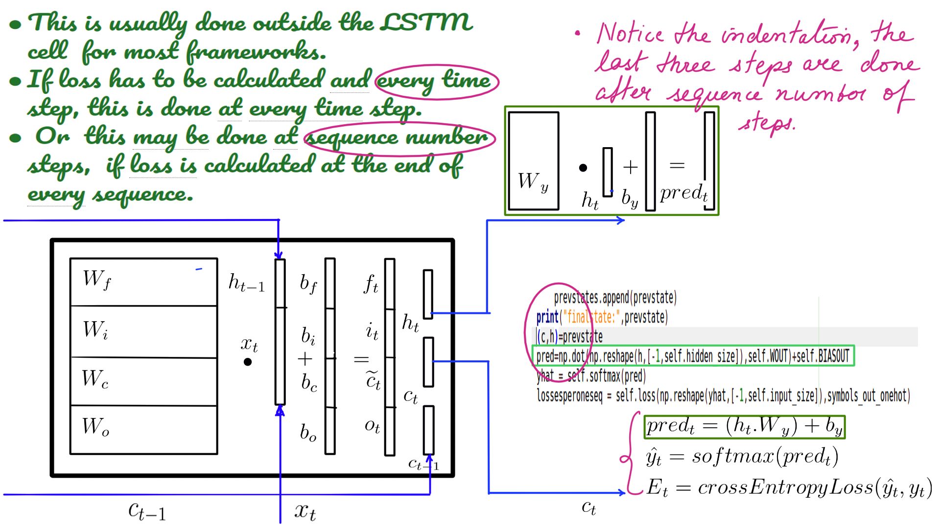
- Usually done internally by “cross_entropy_loss” function.
- Shown here just so that you get an idea.
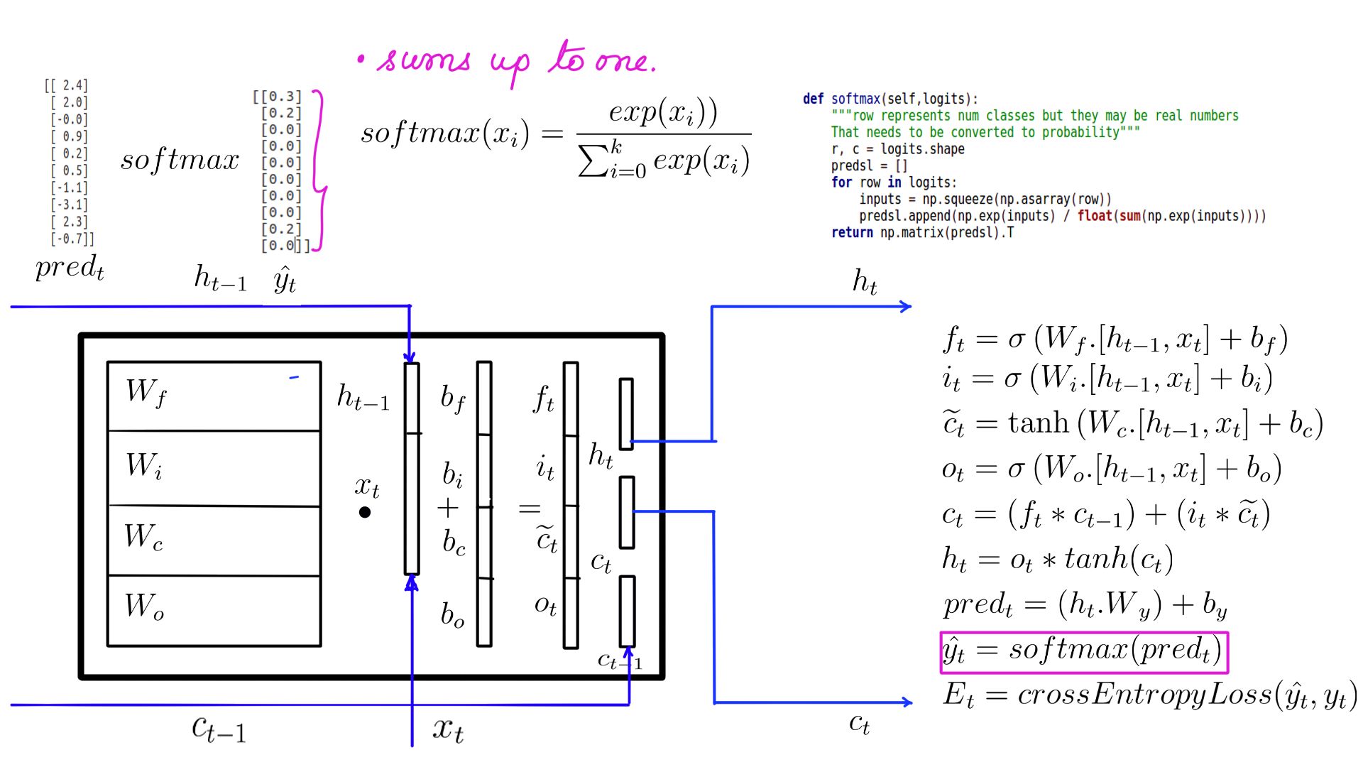
- Does a combination of softmax(figure-12) and loss calculation(figure-13).
- Softmax and a cross_entropy_loss to jog your memory.
- Summary with weights.
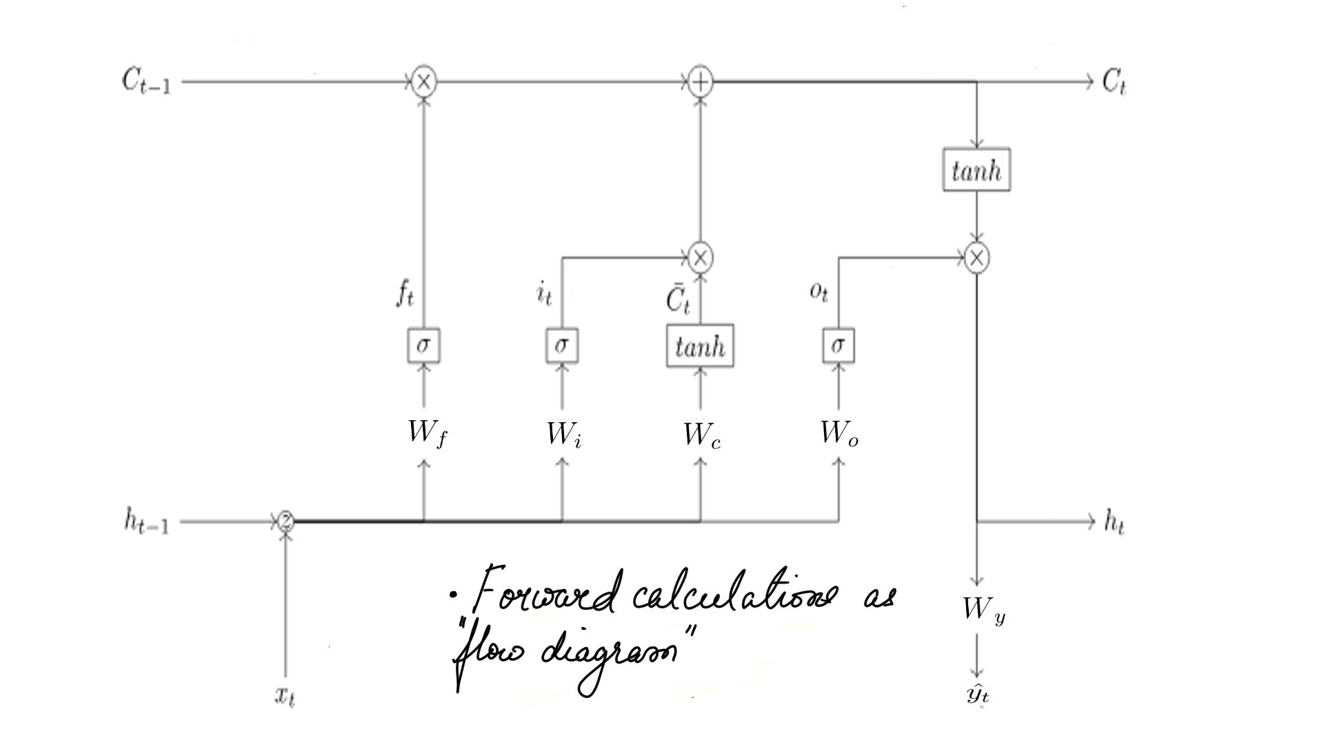
- Summary as flow diagram.
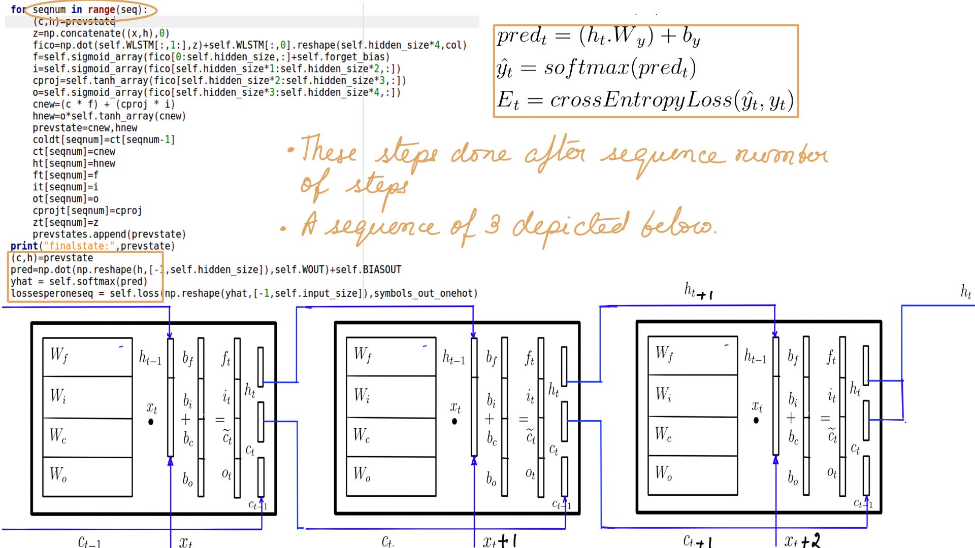
Summary
In summary, then, that was the walk through of LSTM’s forward pass. As a study in contrast, if building a Language model that predicts the next word in the sequence, the training would be similar but we’ll calculate loss at every step. The label would be the ‘X’ just one time-step advanced. However, Let’s not get ahead of ourselves, before we get to a language model, let’s look at the backward pass(Back Propagation) for LSTM in the next post.