Introduction

This is a loss calculating function post the yhat(predicted value) that measures the difference between Labels and predicted value(yhat). Cross entropy is a loss function that is defined as \(\Large E = -y .log ({\hat{Y}})\) where \(\Large E\), is defined as the error, \(\Large y\) is the label and \(\Large \hat{Y}\) is defined as the \(\Large softmax_j (logits)\) and logits are the weighted sum. One of the reasons to choose cross-entropy alongside softmax is that because softmax has an exponential element inside it. A cost function that has an element of the natural log will provide for a convex cost function. This is similar to logistic regression which uses sigmoid. Mathematically expressed as below.

where \(\Large y\) is the label and Yhat is \(\Large \hat{Y}\) the predicted value.

def loss(pred,labels):
  """
  One at a time.
  args:
      pred-(seq=1),input_size
      labels-(seq=1),input_size
  """
  return np.multiply(labels, -np.log(pred)).sum(1)

Listing-1

Above is a loss implementation.

  x = np.array([[1, 3, 5, 7],
                [1,-9, 4, 8]])
  y = np.array([3,1])
  sm=softmax(x)

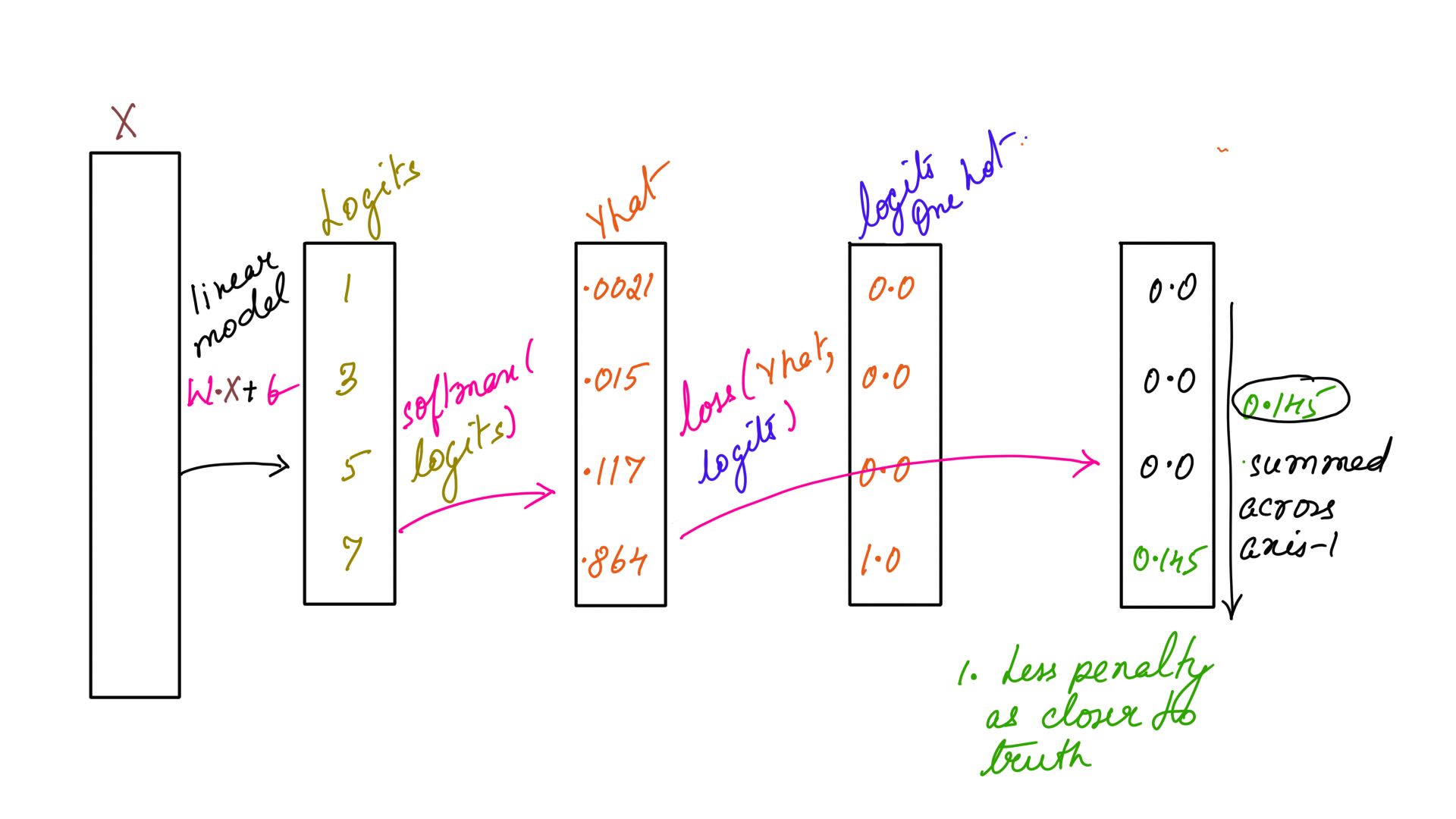
  #prints out 0.145
  print(loss(sm[0],input_one_hot(y[0],4)))
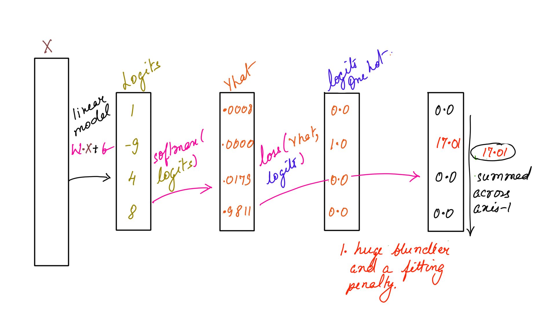
  #prints out 17.01
  print(loss(sm[1],input_one_hot(y[1],4)))

Listing-2

As you can see the loss function accepts softmaxed input and one-hot encoded labels which is being passed in Listing-2. The output is illustrated in figure-1 and 2 below.

• Loss function: Example-1

• Loss function: Example-2

CrossEntropyLoss

CrossEntropyLoss Function is the same loss function above but simplified and adapted for calculating the loss for multiple time steps as is usually required in RNNs. In fact, it calls the same loss function internally. In the above example, we are making 2 comparisons because we are passing 2 sets of logits(x) and 2 labels(y). The labels further have to be adapted into a one-hot of 4 so that they can be compared. Assuming that the above 2 comparisons are for 2 timesteps, the above results can be achieved by calling the CrossEntropyLoss function that calculates the softmax internally.

def cross_entropy_loss(pred,labels):
    """
    Does an internal softmax before loss calculation.
    args:
        pred- batch,seq,input_size
        labels-batch,seq(has to be transformed before comparision with preds(line-133).)
    """
    checkdatadim(pred,3)
    checkdatadim(labels,2)
    batch,seq,size=pred.shape
    yhat=np.zeros((batch,seq,size))

    for batnum in range(batch):
        for seqnum in range(seq):
            yhat[batnum][seqnum]=softmax(np.reshape(pred[batnum][seqnum],[-1,size]))
    lossesa=np.zeros((batch,seq))
    for batnum in range(batch):
        for seqnum in range(seq):
            lossesa[batnum][seqnum]=loss(np.reshape(yhat[batnum][seqnum],[1,-1]),input_one_hot(labels[batnum][seqnum],size))
    return yhat,lossesa

Listing-3

The point to keep in mind is, it accepts it’s 2 inputs in 3(batch,seq,input_size) and 2(batch,seq) dimensions respectively. Batch size usually indicates multiple parallel input sequences, can be ignored for now and be assumed as 1. The shape of pred in our case is batch=1,seq=2,input_size=4. And the shape of labels is batch=1, seq=2. This is illustrated in Listing-3 and Listing-4

  x = np.array([[[1, 3, 5, 7],
                [1,-9, 4, 8]]])
  y = np.array([[3,1]])

  #prints array([[ 0.14507794, 17.01904505]]))
  softmaxed,loss=cross_entropy_loss(x,y)
  print("loss:",loss)

Listing-4

As illustrated in Listing-3 and Listing-4Deep-Breathe version of cross_entropy_loss function returns a tuple of softmaxed output that it calculates internally(only for convenience) and the Loss. The calculated loss, as expected, is the same as before as was while calling the loss function directly.

CrossEntropyLoss Derivative

One of the tricks I have learnt to get back-propagation right is to write the equations backwards. This becomes especially useful when the model is more complex in later articles. A trick that I use a lot.

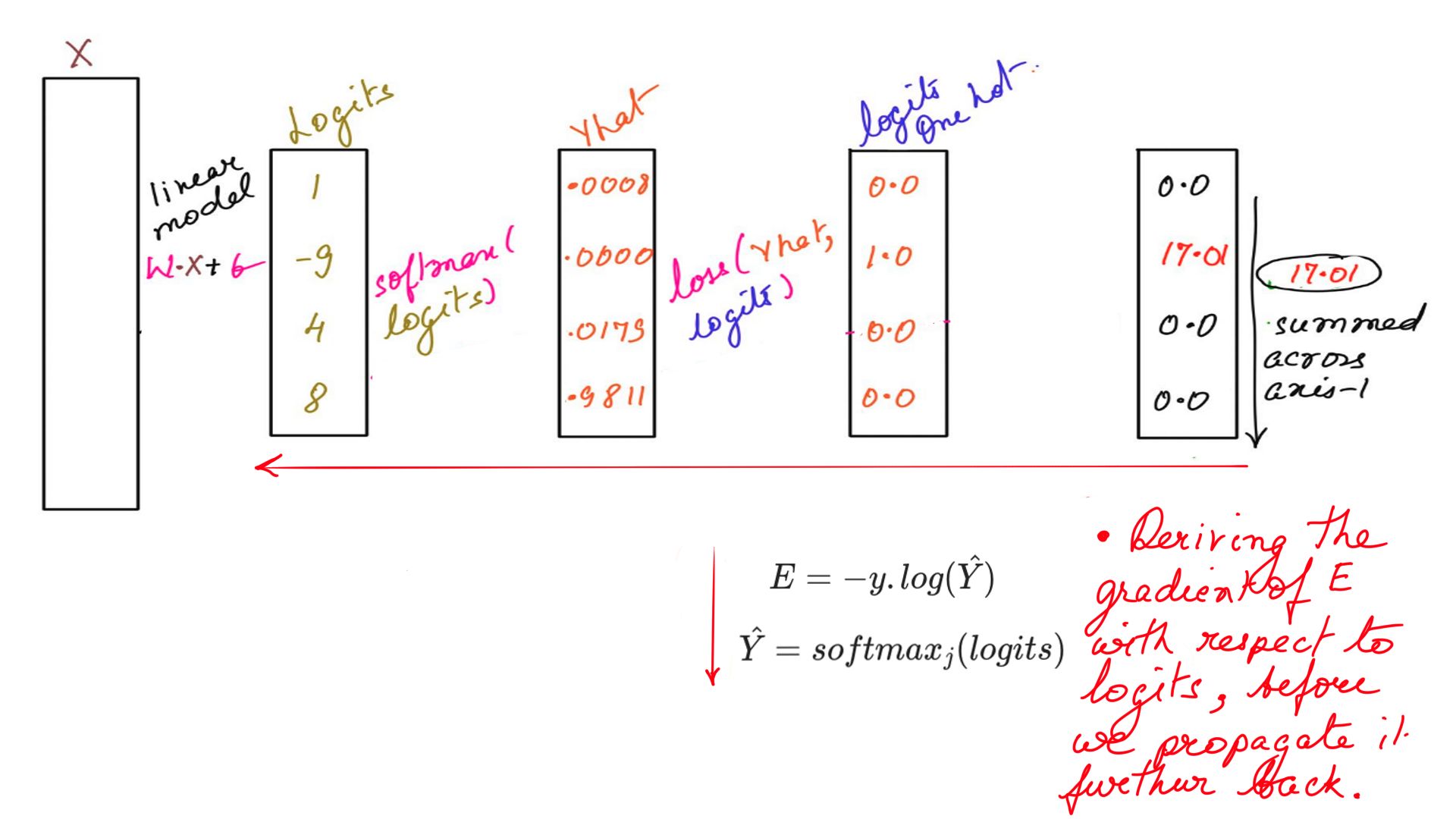
The above equation is written like so below while calculating the gradients.

• Gradient: Example-3

• Deriving the gradients now.

• For calculating \(\Large \frac{\partial {\hat{Y}}}{\partial {logits}}\) where \(\Large \hat{y}\) is the softmax and its derivative is given by eq-1. Combining eq-1 and eq-2.

Since Y is a one hot vector, the term “\(\Large (y + \sum_{i\neq j}y_t)\)” sums up to one.

\(\Large \frac{\partial {E}}{\partial {logits}} = (\hat{y_t} -y) \:\:\:\: eq(3)\)

CrossEntropyLoss Derivative implementation

  softmaxed,loss=cross_entropy_loss(x,y)
  print("loss:",loss)

  batch,seq,size=x.shape
  target_one_hot=np.zeros((batch,seq,size))
  # Adapting the shape of Y
  for batnum in range(batch):
    for i in range(seq):
        target_one_hot[batnum][i]=input_one_hot(y[batnum][i],size)
  dy = softmaxed.copy()
  dy = dy - target_one_hot
  # prints out gradient: [[[ 2.14400878e-03  1.58422012e-02  1.17058913e-01 -1.35045123e-01]
  #                        [ 8.94679461e-04 -9.99999959e-01  1.79701173e-02  9.81135163e-01]]]
  print("gradient:",dy)

Listing-5

Listing-5

Summary

As you can see the idea behind softmax and cross_entropy_loss and their combined use and implementation. Also, their combined gradient derivation is one of the most used formulas in deep learning. Implemented code often lends perspective into theory as you see the various shapes of input and output. Hopefully, cross_entropy_loss’s combined gradient in Listing-5 does the same.