Introduction
LSTMs today are cool. Everything, well almost everything, in the modern Deep Learning landscape is made of LSTMs. I know that might be an exaggeration but, it can only be understated that they are absolutely indispensable. They make up everything directly or indirectly from Time Series(TS) to Neural Machine Translators(NMT) to Bidirectional Encoder Representation from Transformers(BERT) to Neural Turing Machine(NTM) to Differentiable Neural Computers(DNC) etc, and yet they are not very well understood. Whilst there are the elites that write frameworks (Tensorflow, Pytorch, etc), but they are not surprisingly very few in number. The common “Machine learning/Deep Learning” “man/programmer” at best knows how to use it. This is a multi-part series that will unravel the mystery behind LSTMs. Especially it’s gradient calculation when participating in a more complex model like NMT, BERT, NTM, DNC, etc. I do this using the first principles approach for which I have pure python implementation (Deep-Breathe) of most complex Deep Learning models.
What this article is not about?
- This article will not talk about the conceptual model of LSTM, on which there is some great existing material here and here in the order of difficulty.
- This is not about the differences between vanilla RNN and LSTMs, on which there is an awesome, if a somewhat difficult post, by Andrej.
- This is not about how LSTMs mitigate the vanishing gradient problem, on which there is a little mathy but awesome posts here and here in the order of difficulty
What this article is about?
- The reason why understanding LSTM’s inner working is vital is that it underpins the most important models of modern Artificial Intelligence.
- Underpins memory augmented models and architecture.
- Most often it is not used in its vanilla form. There is directionality involved, multiple layers involved, making it a complex moving piece in itself.
- In this multi-part series, I get under the cover of an LSTM using Deep-Breathe especially its back-propagation when it is a part of a more complex model.
Context
Start with the simplest word-generation case-study. We train an LSTM network on a short story. Once trained, we ask it to generate new stories giving it a cue of a few starting words. The focus primarily is on the training process here.
- Picking a starting point in the story that is randomly chosen.
- The training process is feeding in a sequence of n words from the story and checking if (n+1)th word predicted by the model is correct or not. Back propagating and adjusting the weights of the model.
Training Process
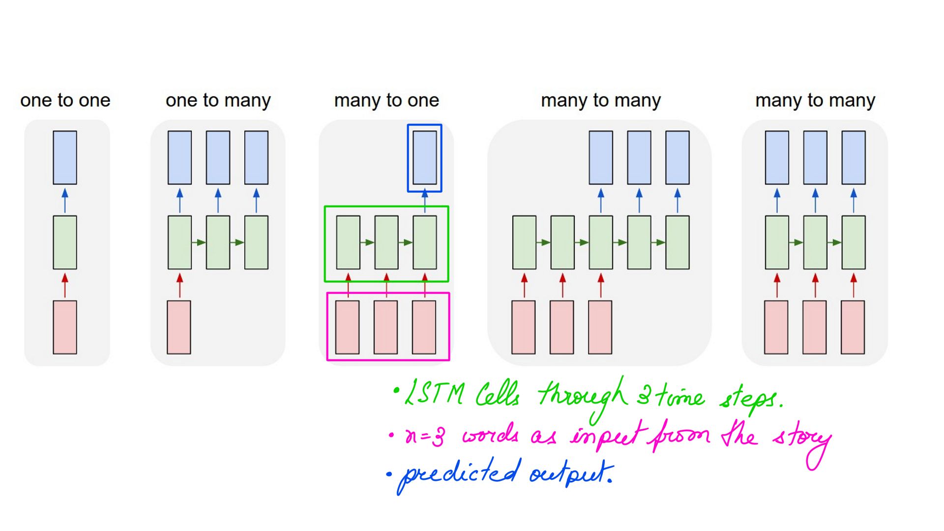
In the next few illustrations we are looking at primary the shape of input, how is the input fed in, when do we check the output before back-propagation happens, etc. All this without looking inside the LSTM Cell just yet. Batch=1(for parallelism), sequence=3(3 words in our example), size=10(vocabulary size 10 so our representation is a one-hot of size 10).
- Sequence of 3 shown below, but that can depend on the use-case.
- Functionally dynamic_rnn feeds in the batches of sequences but its code is written using “tf.while_loop” and not one of python’s native loop construct. With any one of python’s native loop construct only the code within an iteration be optimized on a GPU but with “tf.while_loop” the advantage is that the complete loop can be optimized on a GPU.
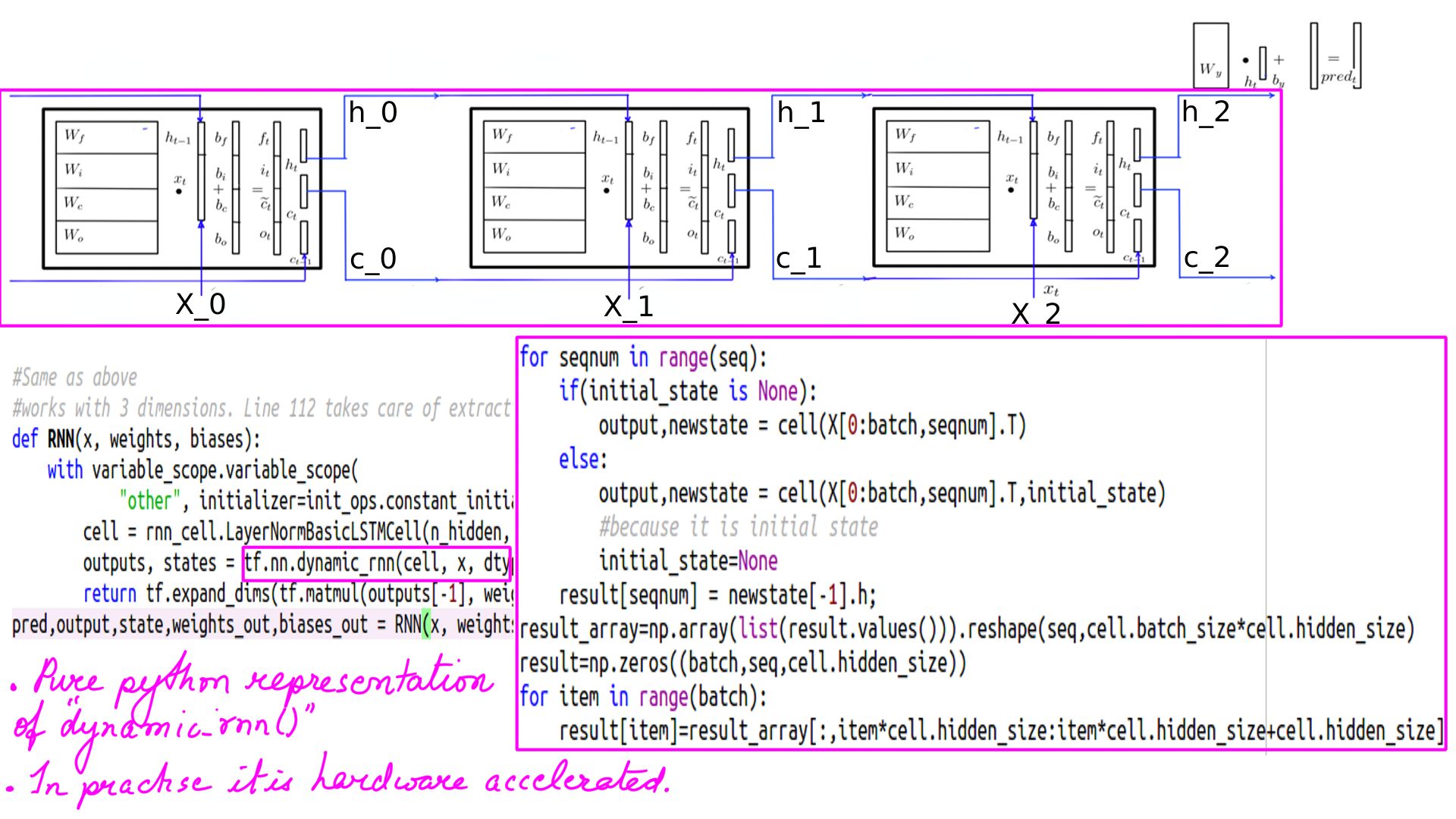
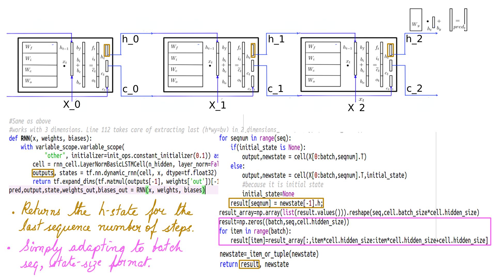
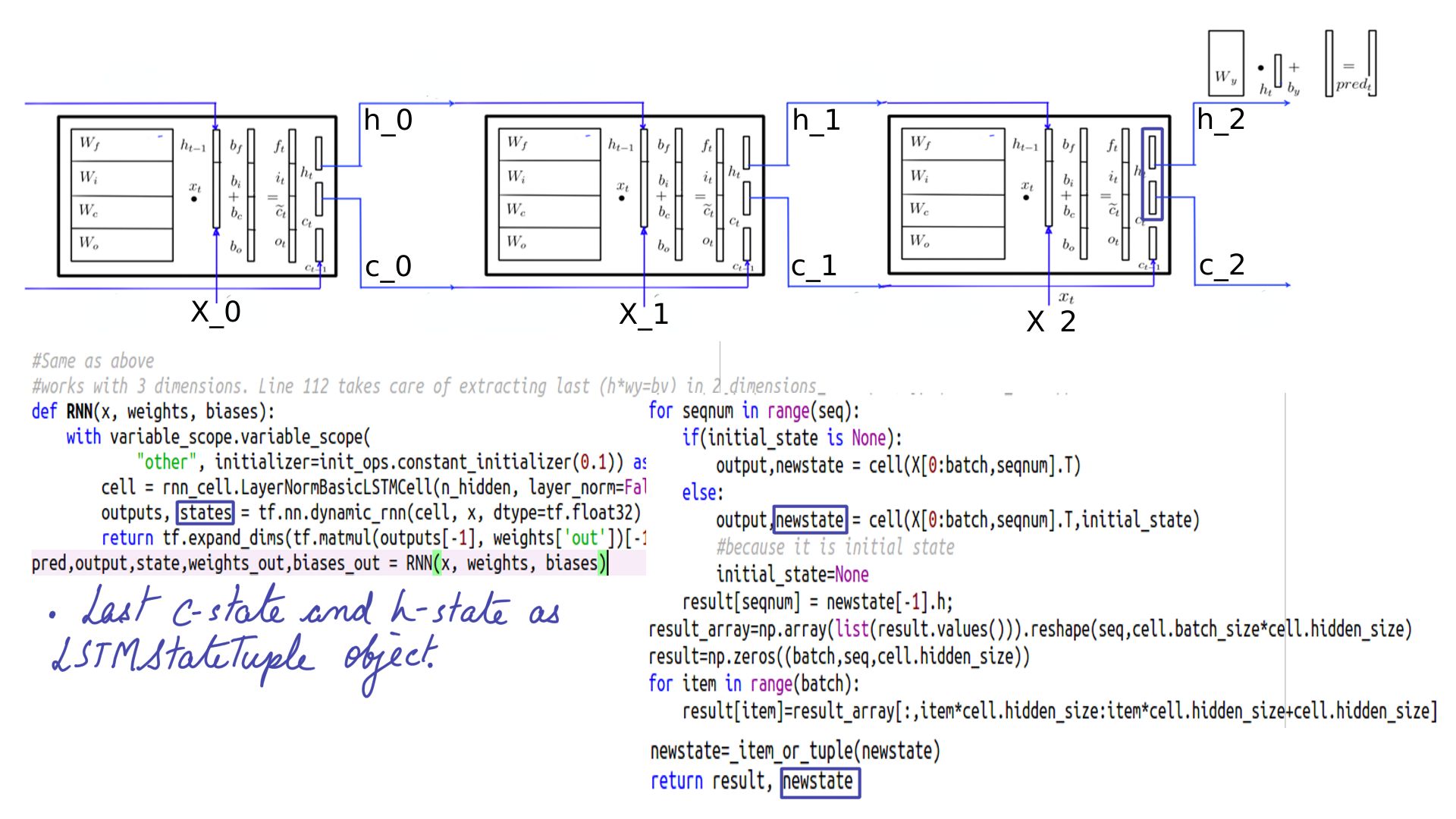
- Returns a tuple of output(H-state across all time steps) and states(C-state and H-state for the last time step).
- Returns a tuple of output(H-state across all time steps) and states(C-state and H-state for the lst time step).
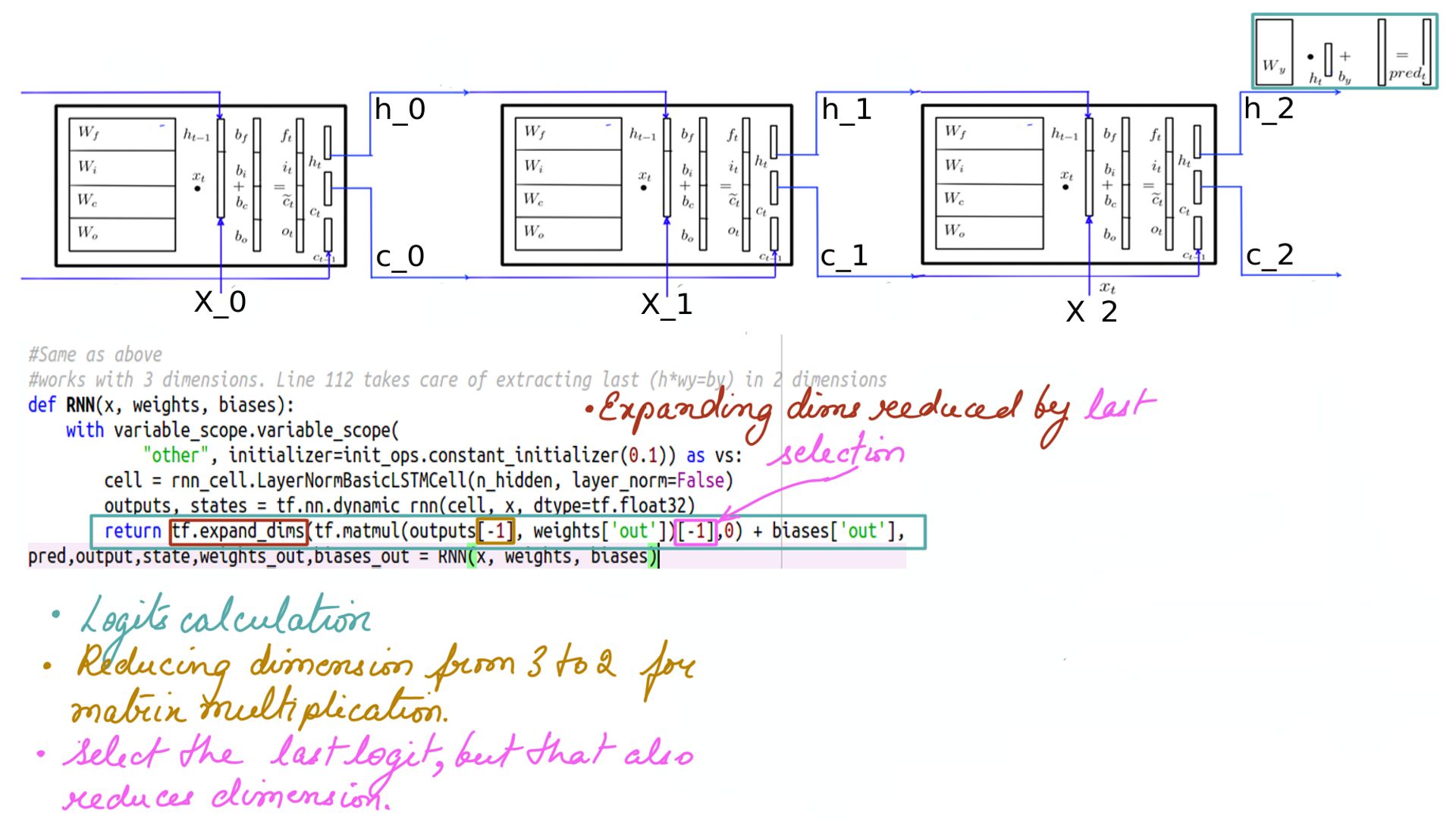
- Multiplier Wy and By which among other things shape the last “h” into the shape of X(10) so a comparison can be made.
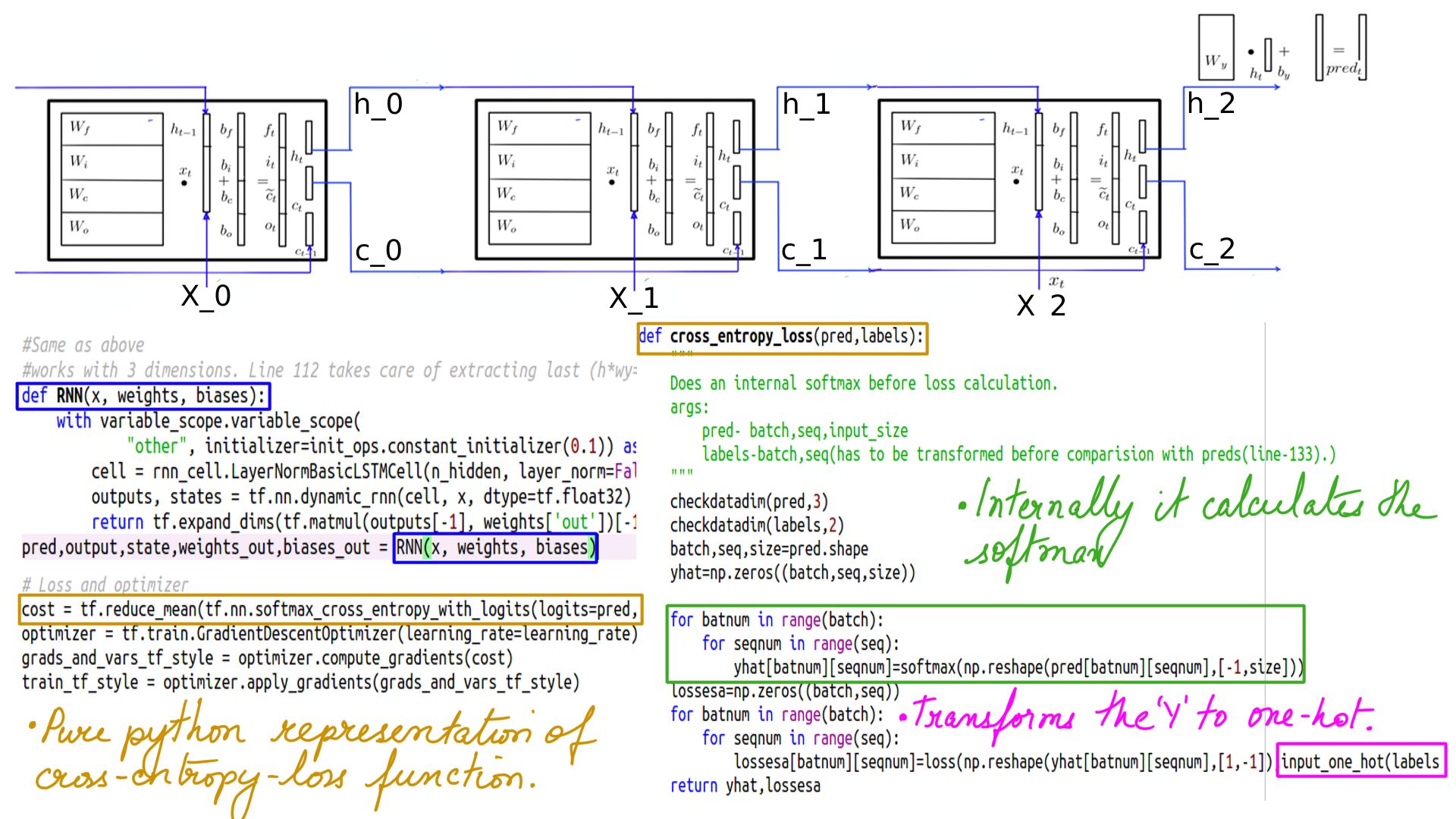
- Finally softmax and cross_entropy_loss.
Quick Comparision between Tensorflow and DEEP-Breathe
This particular branch of DEEP-Breathe has been designed to compare weights with Tensorflow code every step of the way. While there are many reasons, one of the primary reasons for that is understanding. However, this is only possible if both Tensorflow and DEEP-Breathe must start with the same initial weights and their Y-multipliers(Wy and By) must also be identical. Consider the code below.
Tensorflow
1
2
3
4
5
6
7
8
9
10
11
12
13
14
15
16
17
18
19
20
21
22
23
24
25
26
27
28
29
# RNN output node weights and biases
weights = {
'out': tf.Variable([[-0.09588283, -2.2044923 , -0.74828255, 0.14180686, -0.32083616,
-0.9444244 , 0.06826905, -0.9728962 , -0.18506959, 1.0618515 ],
[ 1.156649 , 3.2738173 , -1.2556943 , -0.9079511 , -0.82127047,
-1.1448543 , -0.60807484, -0.5885713 , 1.0378786 , -0.7088431 ],
[ 1.006477 , 0.28033388, -0.1804534 , 0.8093307 , -0.36991575,
0.29115433, -0.01028167, -0.7357091 , 0.92254084, -0.10753923],
[ 0.19266959, 0.6108299 , 2.2495654 , 1.5288974 , 1.0172302 ,
1.1311738 , 0.2666629 , -0.30611828, -0.01412263, 0.44799015],
[ 0.19266959, 0.6108299 , 2.2495654 , 1.5288974 , 1.0172302 ,
1.1311738 , 0.2666629 , -0.30611828, -0.01412263, 0.44799015]]
)
}
biases = {
'out': tf.Variable([ 0.1458478 , -0.3660951 , -2.1647317 , -1.9633691 , -0.24532059,
0.14005205, -1.0961286 , -0.43737876, 0.7028531 , -1.8481724 ]
)
}
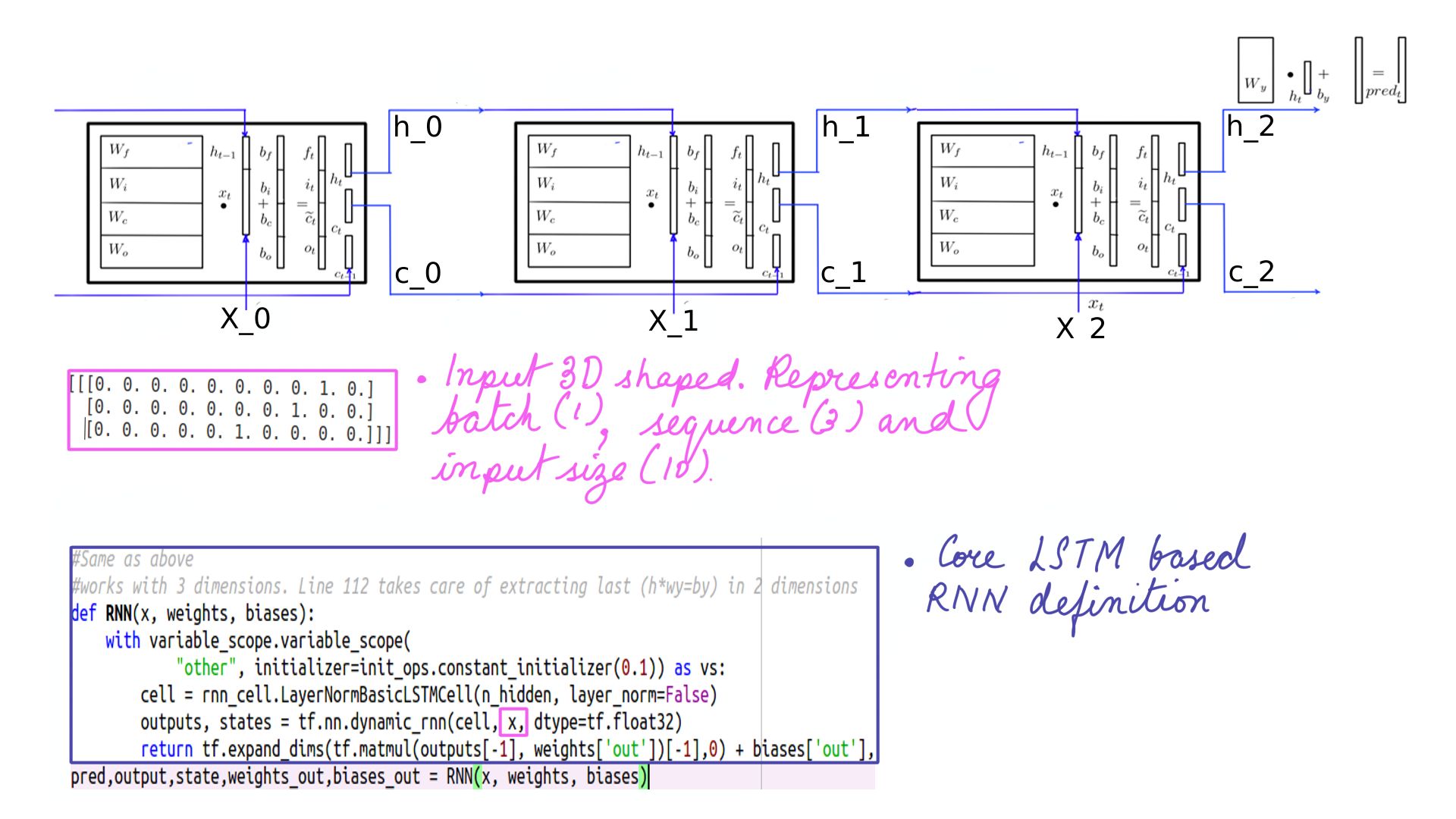
def RNN(x, weights, biases):
with variable_scope.variable_scope(
"other", initializer=init_ops.constant_initializer(0.1)) as vs:
cell = rnn_cell.LayerNormBasicLSTMCell(n_hidden, layer_norm=False)
outputs, states = tf.nn.dynamic_rnn(cell, x, dtype=tf.float32)
return tf.expand_dims(tf.matmul(outputs[-1] , weights['out'])[-1],0) + biases['out'],outputs[-1],states,weights['out'],biases['out']
pred,output,state,weights_out,biases_out = RNN(x, weights, biases)
Listing-1
- The pre-initialized weights and biases in line(2) and line(16) utilized as Wy and By in line(26)
- The internal weights of LSTM initialized in line(22-23)
- Tensorflow graph mode is the most non pythonic design done in python. It sounds crazy but is true. Consider line(21-26), this function gets called multiple times in the training loop and yet the cell(line(24)) is the same cell instance across multiple iterations. Tensorflow in the graph mode builds the DAG first and identifies the cell by the name in that graph. That is source of confusion to most programmers, especially python programmers.
- The complete executable Listing-1 and its execution script.
Deep-Breathe
I could have done without a similar behavior in Deep-Breathe but the programmer in me just could not resist. Especially since I earned my stripes in C/C++ and assembly kind of languages, python proved challenging. Without building a full-fledged graph, I associated the variable name with the corresponding weight, i.e. when the variable name is the same it fetches the same set of weights. This is difficult and not recommended but, if you care to see, then its demonstrated here, here, here and here. To summarize in the Listing-2 there is a single set of weights for the LSTMCell despite getting called multiple times in the loop.
1
2
3
4
5
6
7
8
9
10
11
12
13
14
15
16
17
18
19
20
21
22
23
24
25
def RNN(x, weights, biases):
  with WeightsInitializer(initializer=init_ops.Constant(0.1)) as vs:
      cell = LSTMCell(n_hidden,debug=True)
      result, state = dynamic_rnn(cell, symbols_in_keys)
  "Dense in this case should be out of WeightsInitializer scope because we are passing constants"
  out_l = Dense(10,kernel_initializer=init_ops.Constant(out_weights),bias_initializer=init_ops.Constant(out_biases))
  return out_l(state.h)


def LOSS(X,target):
  pred=RNN(X,out_weights,out_biases)
  return cross_entropy_loss(pred.reshape([1,1,vocab_size]),np.array([[target]]))

while step < training_iters:
  if offset > (len(train_data) - end_offset):
      offset = rnd.randint(0, n_input + 1)
  print("offset:", offset)
  symbols_in_keys = [input_one_hot(dictionary[str(train_data[i])],vocab_size) for i in range(offset, offset + n_input)]
  symbols_in_keys = np.reshape(np.array(symbols_in_keys), [-1, n_input, vocab_size])
  print("symbols_in_keys:",symbols_in_keys)
  target=dictionary[str(train_data[offset + n_input])]
  yhat,cel=LOSS(symbols_in_keys,target)


Listing-2
- The complete executable graph-mode and its execution script.
- The complete executable for non-graph-version and its execution script. To make Tensorflow more pythonic, they have enabled eager mode and will be the default going forward especially from Tensorflow 2.0 onwards. However, major project as on today is still on the older version.
Summary
In summary, then, that was the walk through of code surrounding LSTM training, without getting into LSTM or its weights just yet. That would be the topic of our next article.