Introduction

In this multi-part series (part-1,part-2,part-3), we look into composing LSTM into multiple higher layers and its directionality. Though Multiple layers are compute-intensive, they have better accuracy and so does bidirectional connections. More importantly, a solid understanding of the above mentioned paves the way for concepts like Highway connections, Residual Connections, Pointer networks, Encoder-Decoder Architectures and so forth in future article. I do this using the first principles approach for which I have pure python implementation Deep-Breathe of most complex Deep Learning models.

What this article is not about?

• This article will not talk about the conceptual model of LSTM, on which there is some great existing material here and here in the order of difficulty.
• This is not about the differences between vanilla RNN and LSTMs, on which there is an awesome, if a somewhat difficult post, by Andrej.
• This is not about how LSTMs mitigate the vanishing gradient problem, on which there is a little mathy but awesome posts here and here in the order of difficulty

What this article is about?

• Using the first principles we picturize/visualize MultiRNNCell and Bidirectional RNNs and their backward propagation.
• Then we use a heady mixture of intuition, Logic, and programming to prove mathematical results.

Context

This is the same example and the context is the same as described in part-1. The focus. however, this time is on MultiRNNCell and Bidirectional RNNs.

There are 2 parts to this article.

1. Multi layer RNNs
2. Bidirectional RNNs
3. Combining Bidirectional and MultiLayerRNNs

Multi layer RNNs

1. Recurent depth
2. Feed Forward depth
3. Multi layer RNNs Forward pass
4. Multi layer RNNs backward propagation

Recurent depth

A quick recap, LSTM encapsulates the internal cell logic. There are many variations to Cell logic, VanillaRNN, LSTMs, GRUs, etc. What we have seen so far is they can be fed with sequential time series data. We feed in the sequence, compare with the labels, calculate errors back-propagate and adjust the weights. The length of the fed in the sequence is informally called recurrent depth.

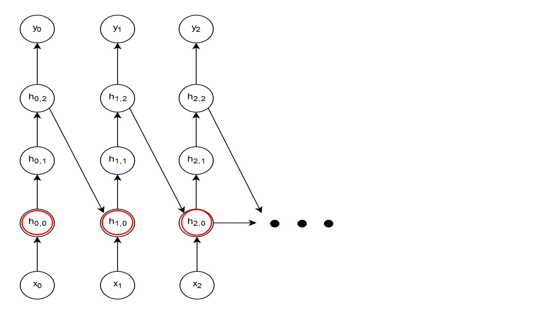
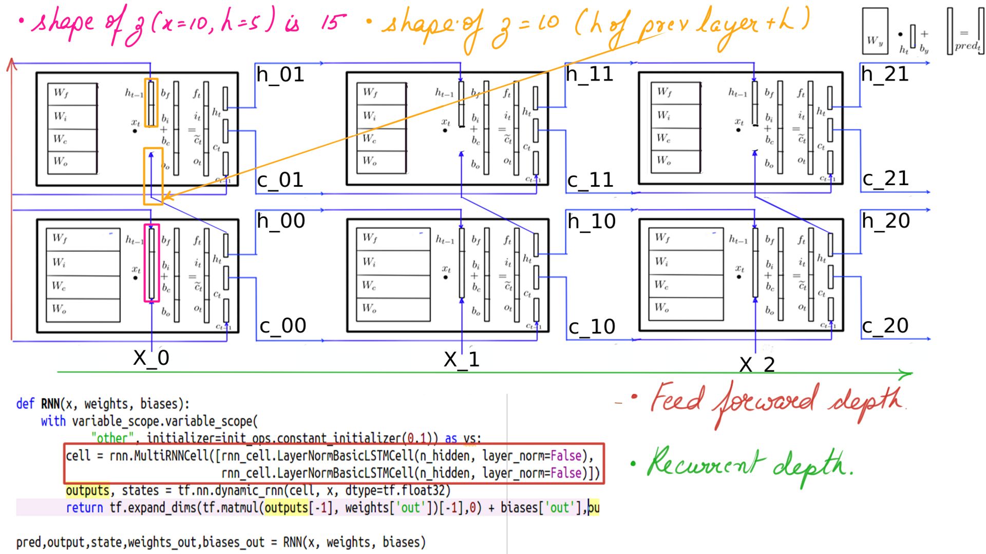
Figure-1 shows the recurrent depth. Formally stated, Recurrent depth is the Longest path between the same hidden state in successive time-steps. The recurrent depth is amply clear.

Feed Forward depth

The topic of this article is Feed-forward depth, more akin to the depth we have in vanilla neural networks. It is the depth of a network that is generally attributed to the success of deep learning as a technique. There are downsides too, too much compute budget for one if done indiscriminately. That being said, well look at the inner workings of Multiple layers and how we set it up in code.

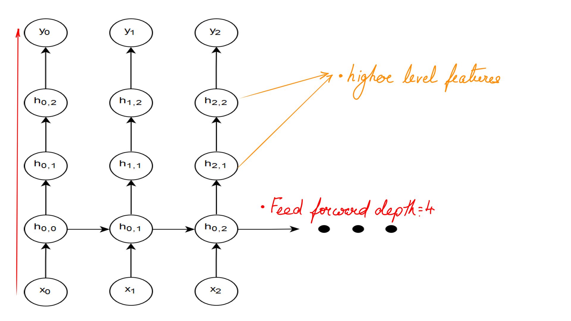
Figure-2 shows the Feed-Forward depth. Formally stated the longest path between an input and output at the same timestep.

Multi layer RNNs Forward pass

For the most part this straight forward as you have already seen in the previous article in this series. The only difference is that there are multiple cells(2 in this example) now and how the state flows forward and gradient flows backwards.

• MultiRNNCell forward pass summary.

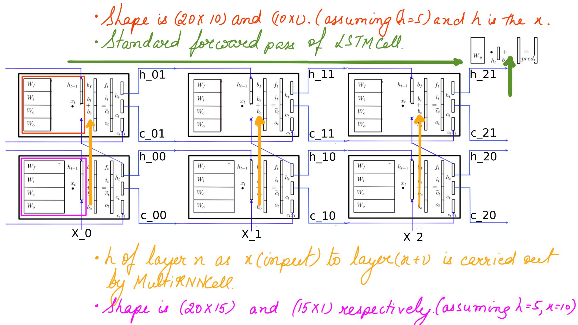
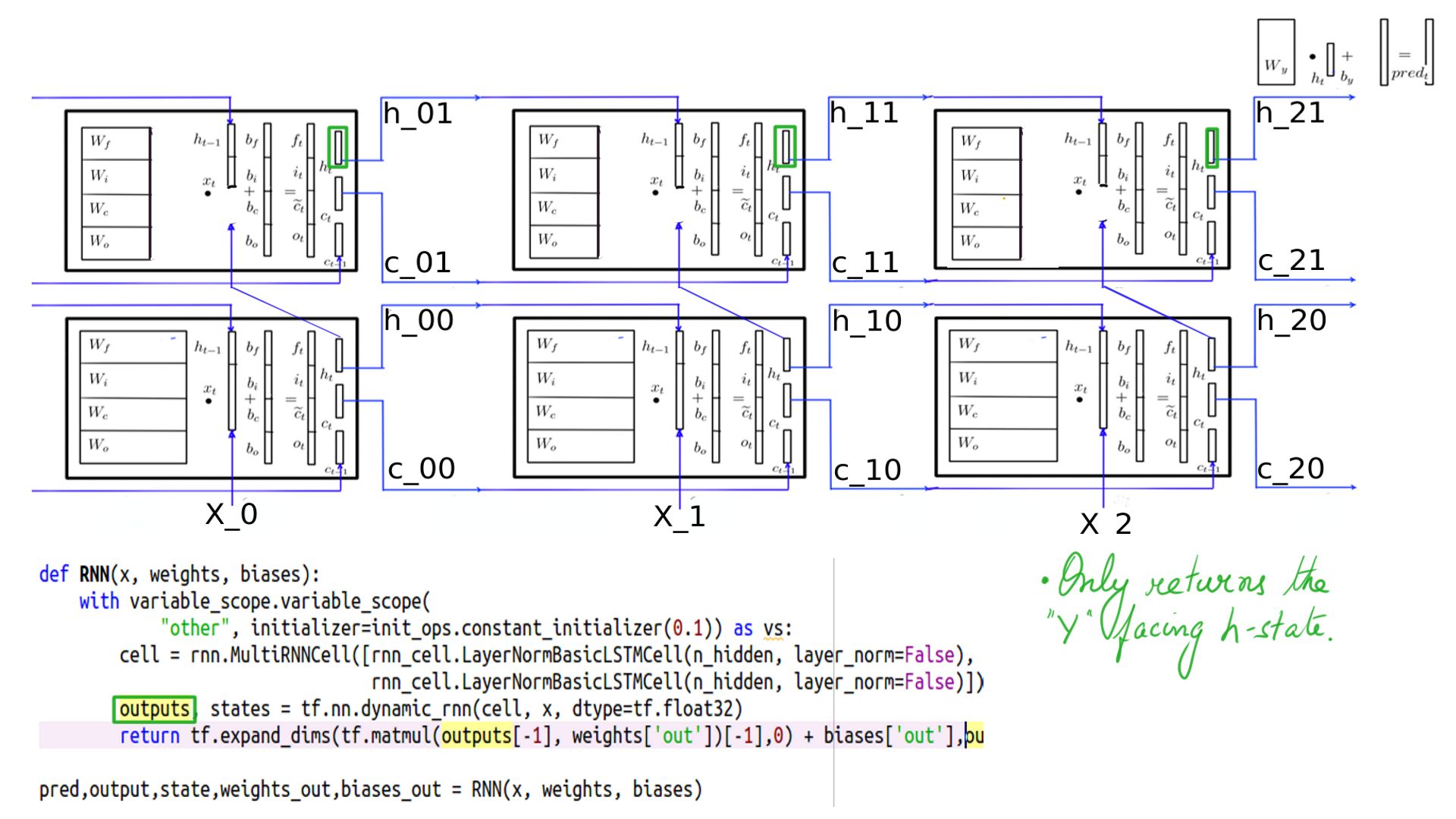
• Multi-layer RNNs Forward pass
• Notice the state being passed(yellow) from the first layer to the second.
• The softmax and cross_entropy_loss are done on the second layer output expectedly.

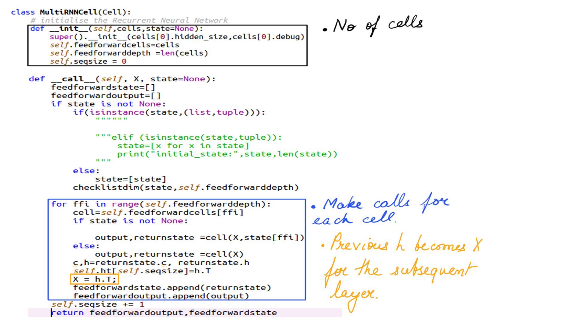
• Complete code of MultiRNNCell from DEEP-Breathe helps in looking at the internals

• MultiRNNCell outputs returned

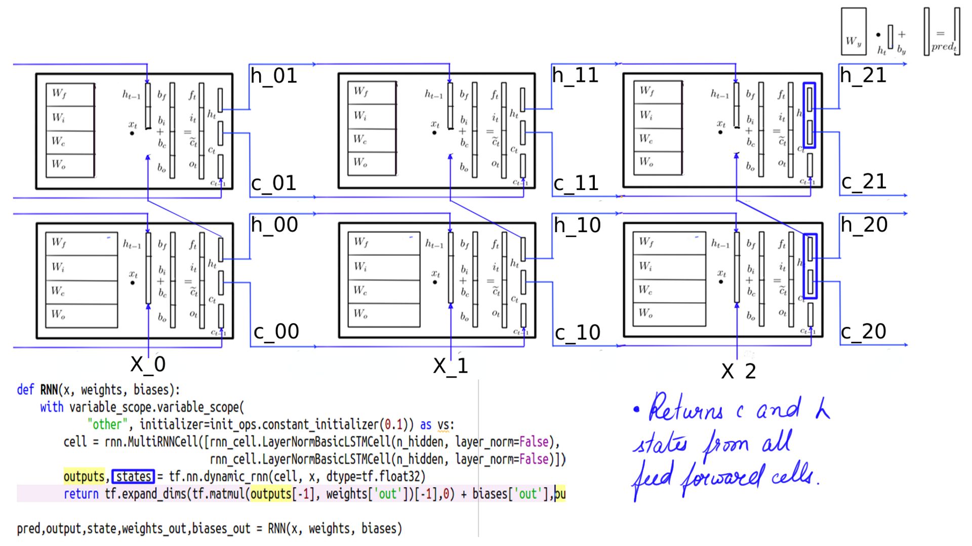
• MultiRNNCell states returned

Also when using Deep-Breathe you could enable forward or backward logging for MultiRNNCell like so

  cell= MultiRNNCell([cell1, cell2],debug=True,backpassdebug=True)
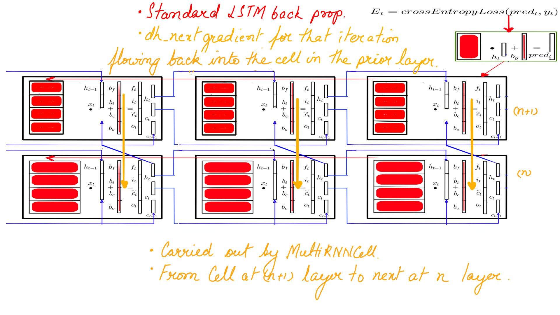
  Listing-1

Multi layer RNNs backward propagation

Again, for the most part, this is almost identical to standard LSTM Backward Propagation which we went through in detail in part-3. So if you have got a good hang of it, only a few things change. But before we go on, refresh DHX and the complete section before you resume here. Here is what we have to calculate.

• MultiRNNCell Backward propagation summary.

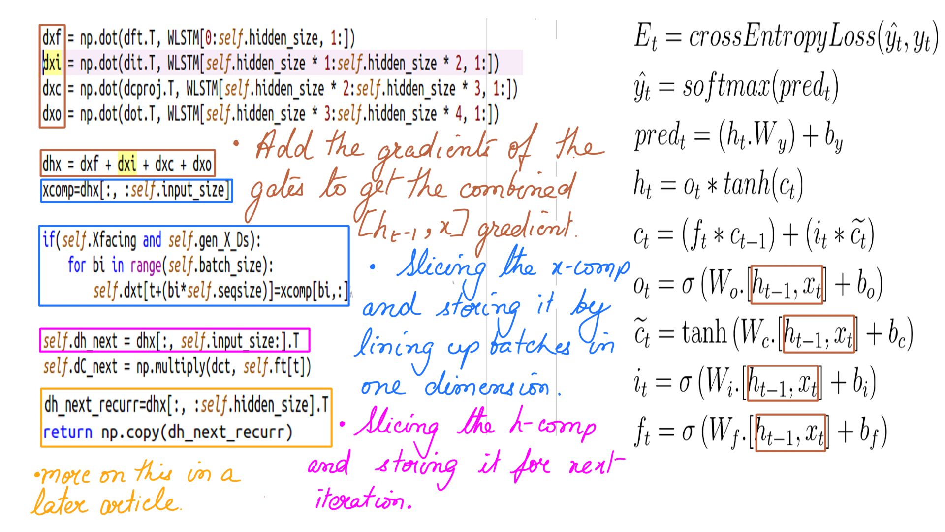
I’ll reproduce DHX here just to set the context and note down the changes.

Standard DHX for Regular LSTM Cell

• Dhx, Dh_next, dxt.
• Complete listing can be found at code-1

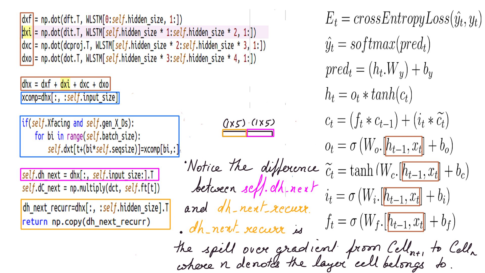
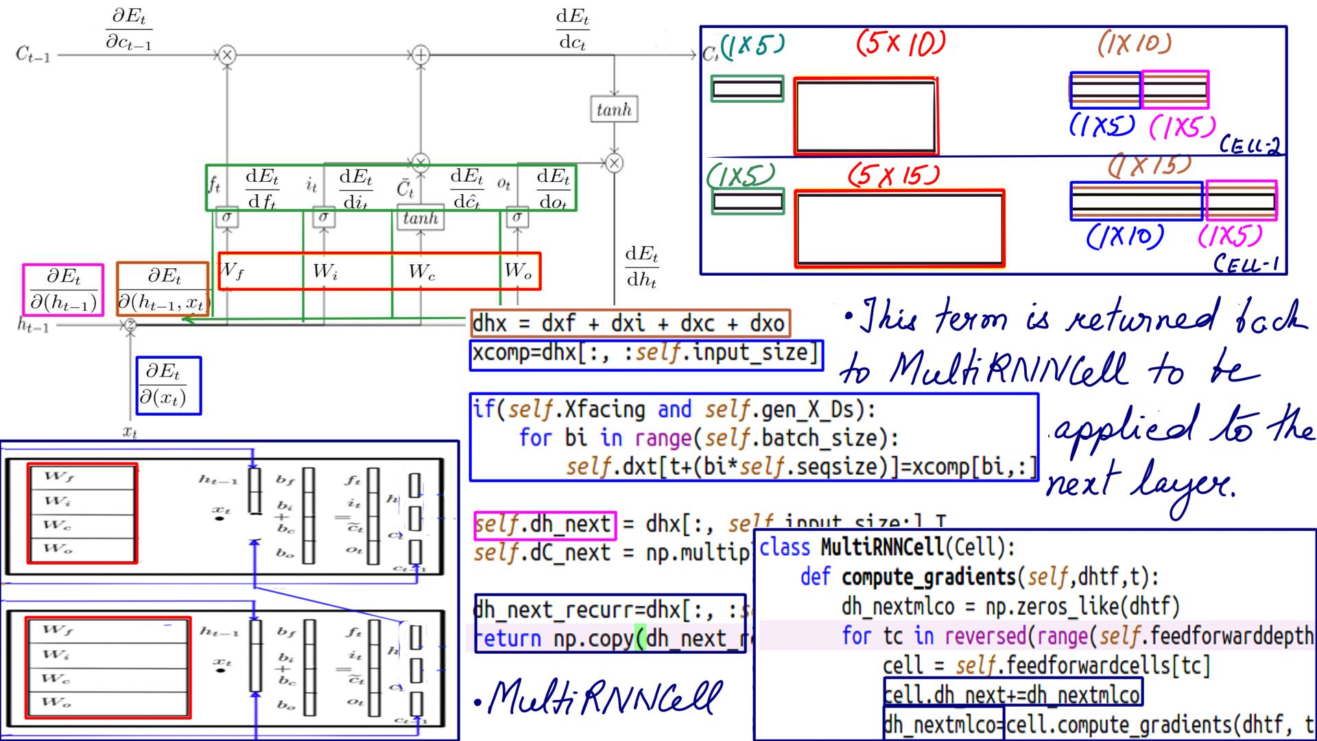
DHX for MultiRNNCell composing LSTM Cell

• Dhx, Dh_next, dxt as usual and then dh_next_recurr which is passed back to MultiRNNCell to be applied to the next layer.
• Complete listing can be found at code-1. Pay careful attention to the weights shapes.

Standard DHX schematically Regular LSTM Cell

• Many models like Neural Machine Translators(NMT), Bidirectional Encoder Representation from Transformers(BERT) use word embeddings as their inputs(Xs) which oftentimes need learning and that is where we need dxt

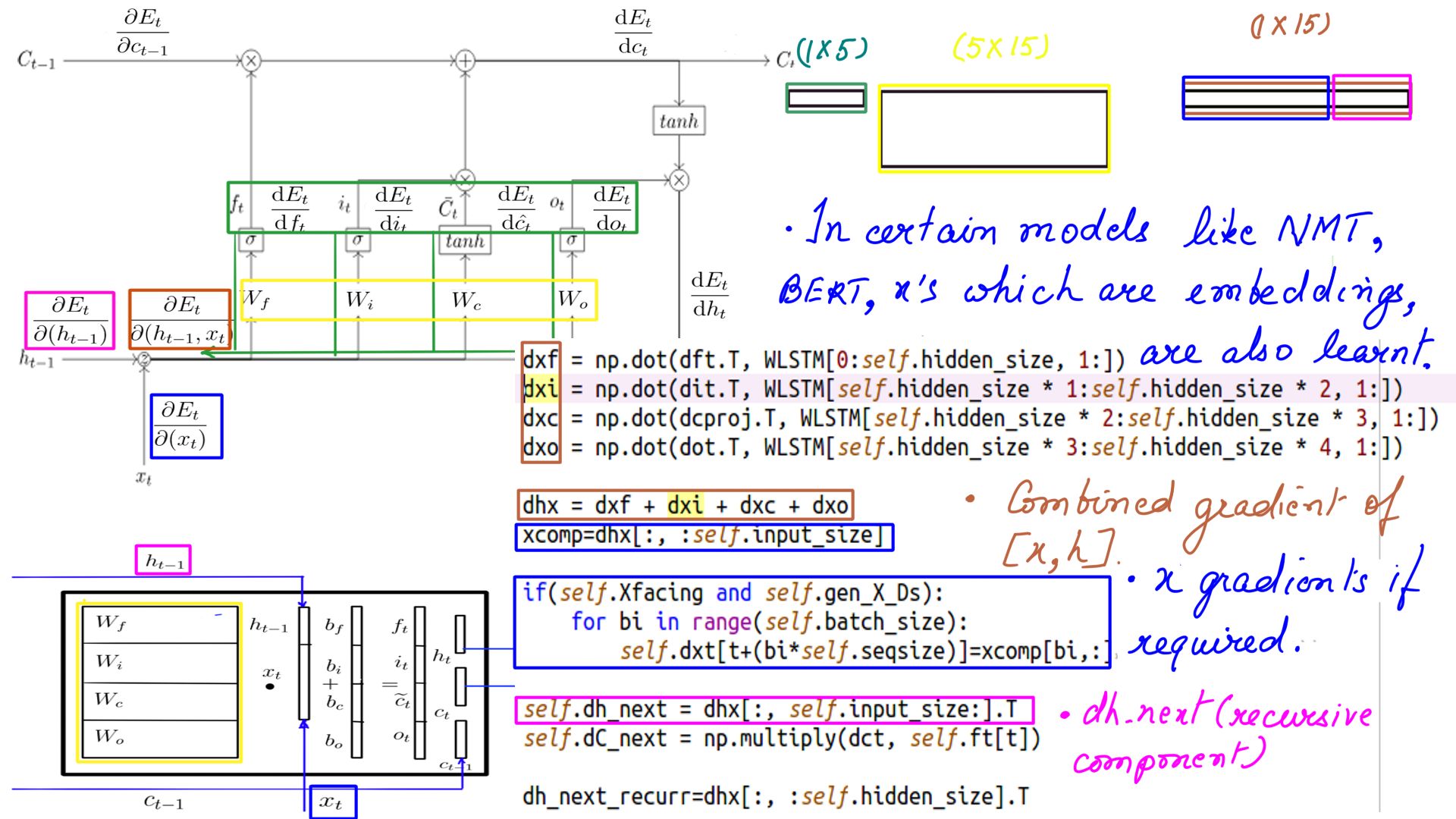
DHX schematically for MultiRNNCell composing LSTM Cell

• Dhx, Dh_next, dxt as usual and then dh_next_recurr which is passed back to MultiRNNCell to be applied to the next layer.
• The Complete listing can be found at code-1, in particular, the MultiRNNCell “compute_gradient()”. Pay careful attention to the weights’ shapes.

Bidirectional RNNs

The bidirectional RNNs are great for accuracy but the compute budget goes up. Most advanced architectures use bidirectional for better accuracy. It has 2 cells or 2 multi-cells where the sequence is fed in forwards as well as backwards. For many sequences, language models for instance, when the sequence is fed in-reverse then it provides a bit more context of what is being said. Consider the below statements.

• One of the greatest American Richard Feynman said. “If I could explain it to the average person, it wouldn’t have been worth the Nobel Prize.”
• One of the greatest American Richard Pryor said. “I became a performer because it was what I enjoyed doing.”

The first six words of the 2 sentences are identical. But if this sequence was fed in backwards as well, then the context would have been much clearer. Setting it up much easier as illustrated in the next few figures.

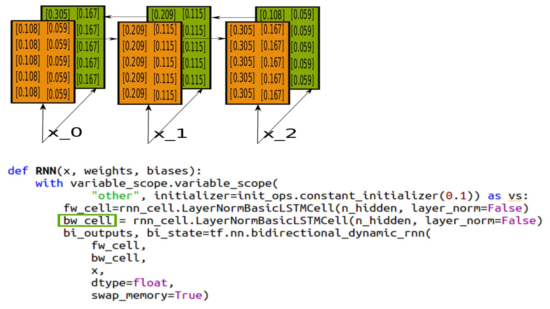
• Bidirectional RNNs.
• Simple 2 separate cells fed in with the same sequence in opposite directions.

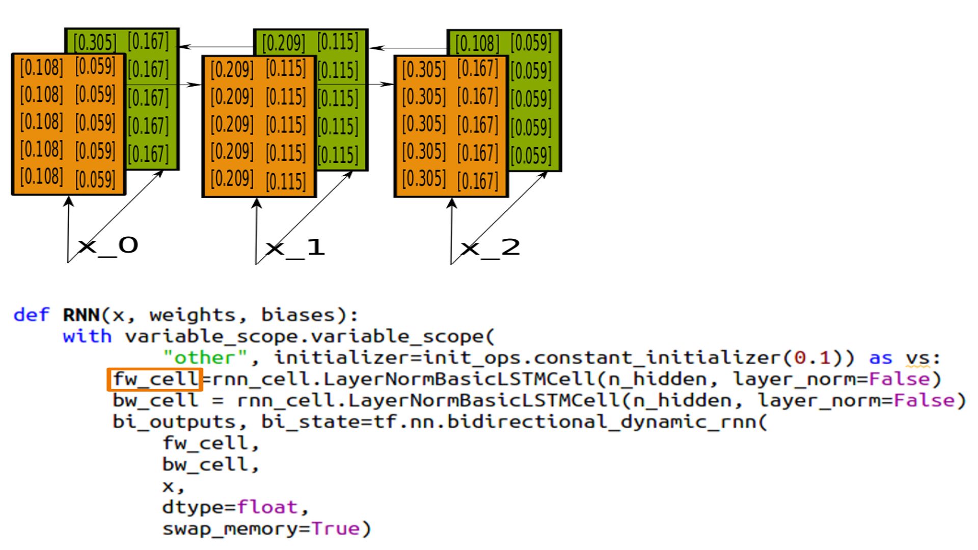
• Bidirectional RNNs
• The State looks identical but reversed, and that is because they have been initialized identically for comparison purposes. In practice we don’t do that.

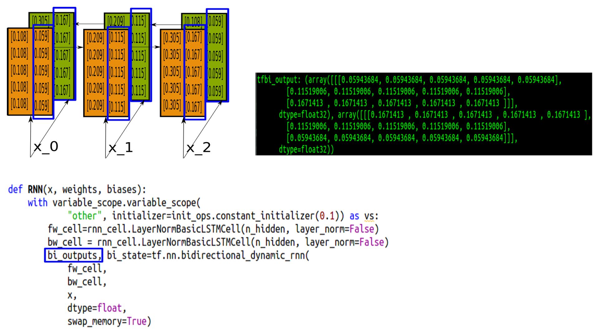
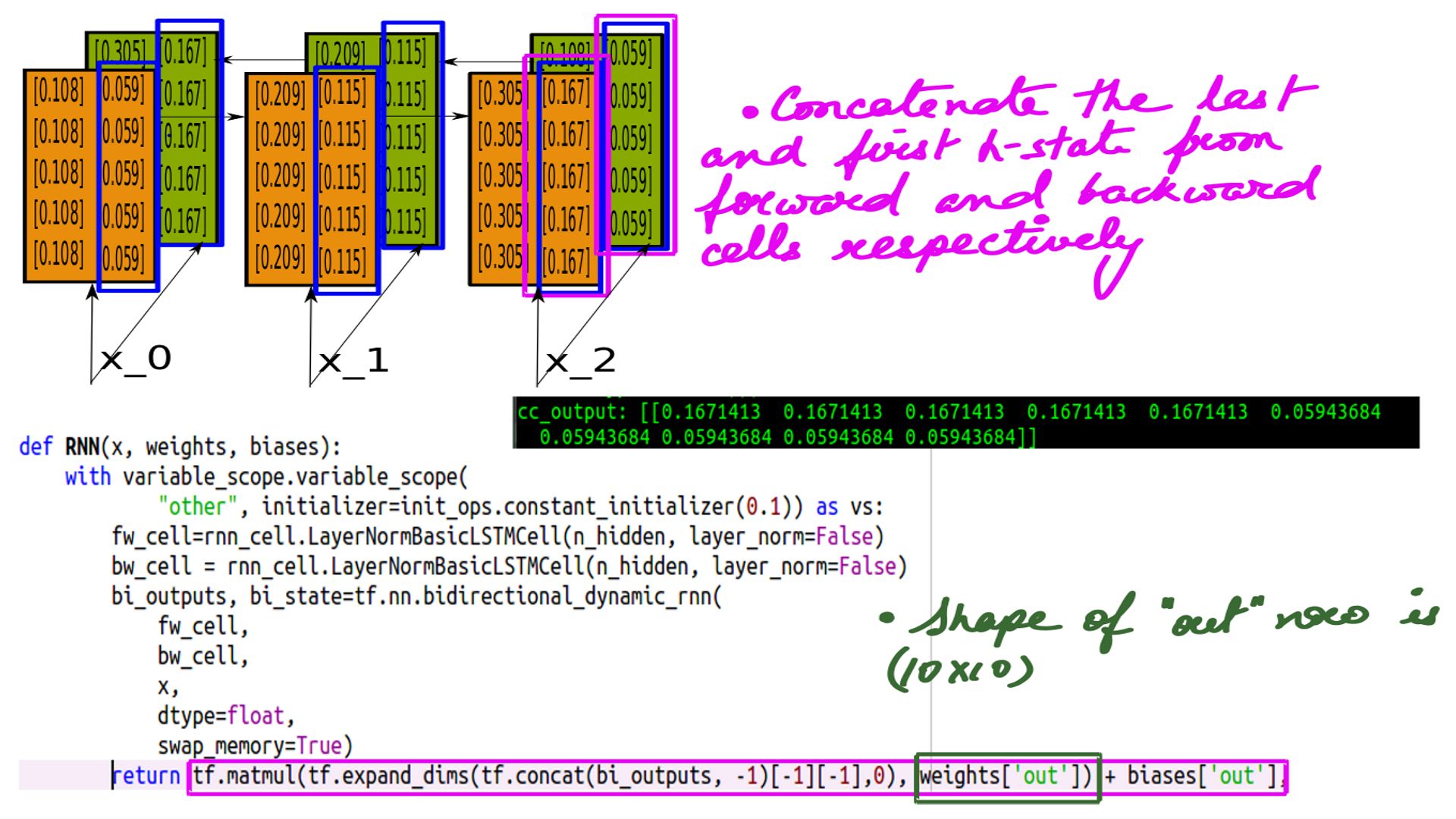
• Bidirectional RNNs Output
• Tupled h-states for both the cells.

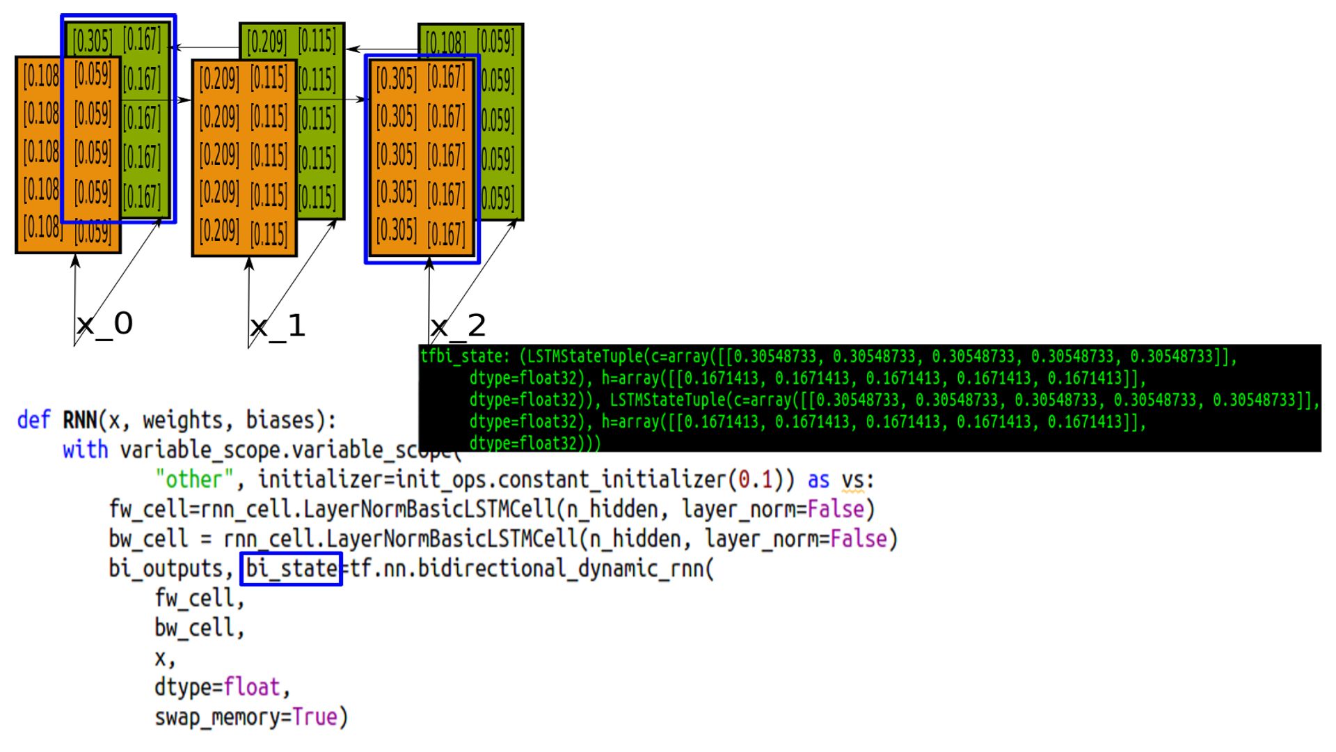
• Bidirectional RNNs States
• Tupled and last (c-state and h-state) for both the cells.

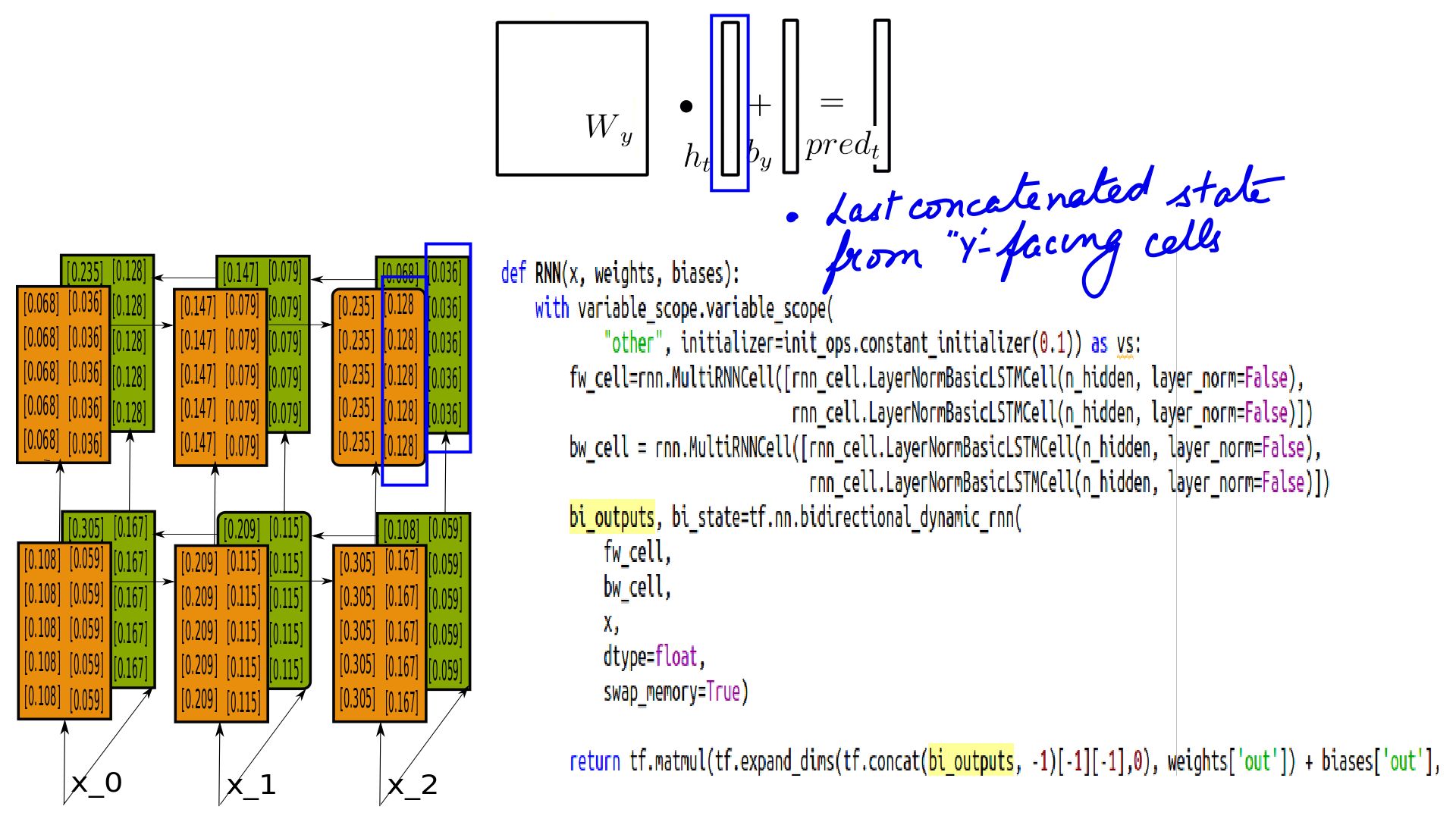
• Bidirectional RNNs Pred Calculation
• Pred calculation is similar except the last h-state is concatenated changing the shape of Wy.

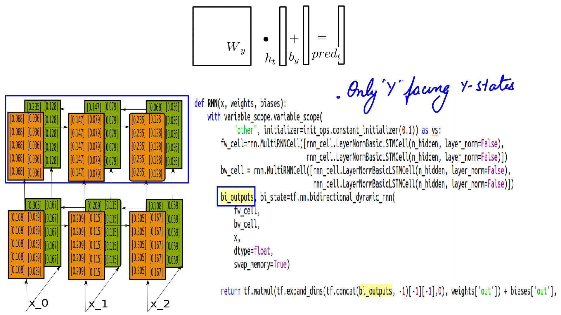
Combining Bidirectional and MultiLayerRNNs

• Combining Bidirectional RNNs and MultiRNNCell Output.

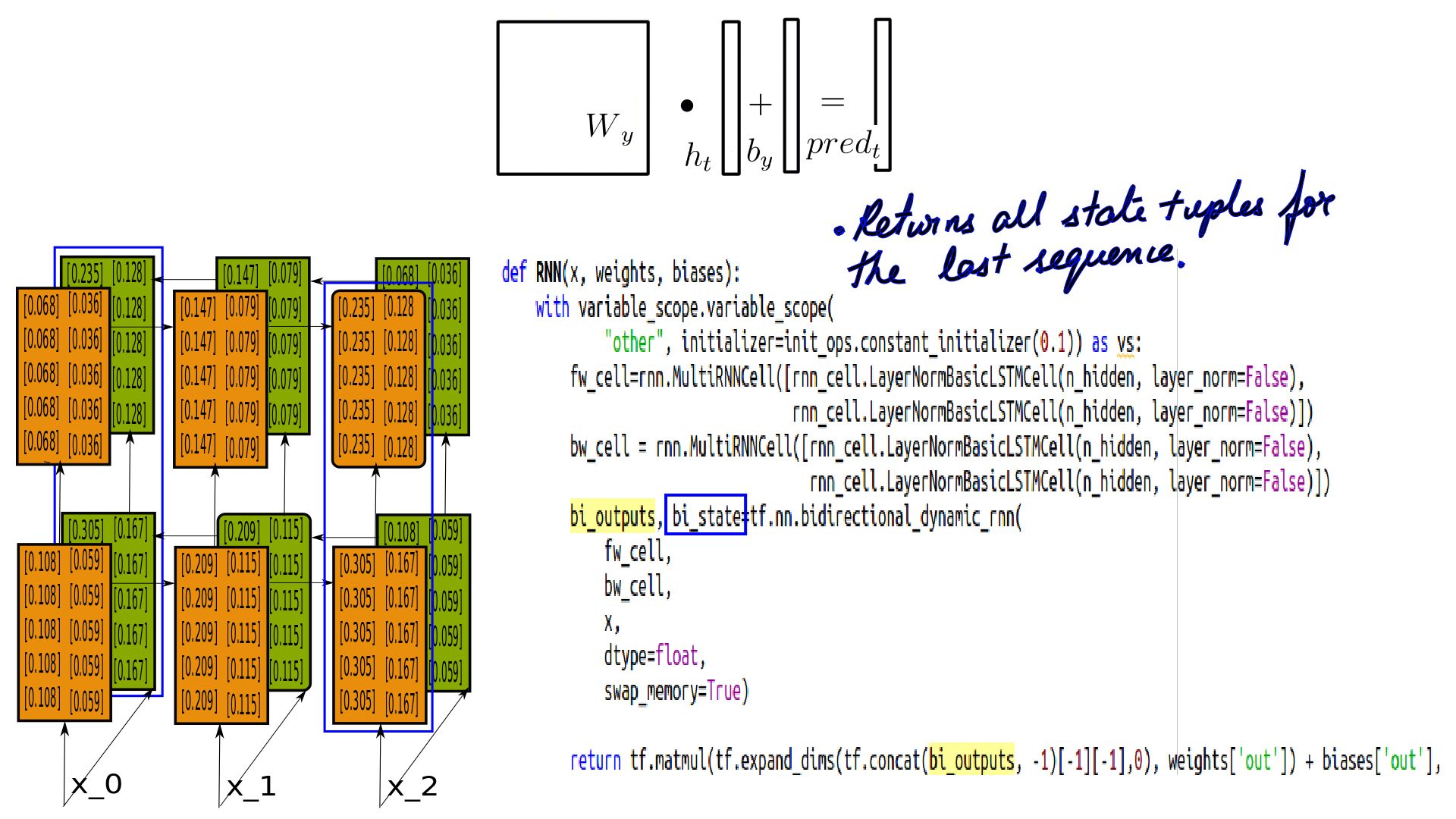
• Combining Bidirectional RNNs and MultiRNNCell State.

• Combining Bidirectional RNNs and MultiRNNCell Pred Calculation.

Summary

Finally, that would be the complete documentation of LSTMs inner workings. Maybe a comparison with RNNs for vanishing gradient improvement will complete it. But that apart, once we have a drop on LSTMs like we did, using them in more complex architectures will become a lot easier. In the immediate next article, we’ll look at the improvements in propagation because of vanishing and exploding gradients, if any, brought about by LSTMs over RNNs.